Software Evolution and Maintenance A Practitioner’s Approach Chapter

63 Slides2.56 MB
Software Evolution and Maintenance A Practitioner’s Approach Chapter 6 Impact Analysis Software Evolution and Maintenance (Chapter 6: Impact Analysis) Tripathy & Naik
Outline of the Chapter 6.1 General Idea 6.2 Impact Analysis Process 6.2.1 Identifying the SIS 6.2.2 Analysis of Traceability Graph 6.2.3 Identifying the Candidate Impact Set 6.3 Dependency-based Impact Analysis 6.3.1 Call Graph 6.3.2 Program Dependency Graph 6.4 Ripple Effect 6.4.1 Computing Ripple Effect 6.5 Change Propagation Model 6.5.1 Recall and Precision of Change Propagation Heuristics 6.5.2 Heuristics for Change Propagation 6.5.3 Empirical Studies Software Evolution and Maintenance (Chapter 6: Impact Analysis) Tripathy & Naik
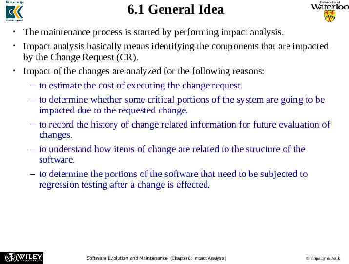
6.1 General Idea The maintenance process is started by performing impact analysis. Impact analysis basically means identifying the components that are impacted by the Change Request (CR). Impact of the changes are analyzed for the following reasons: – to estimate the cost of executing the change request. – to determine whether some critical portions of the system are going to be impacted due to the requested change. – to record the history of change related information for future evaluation of changes. – to understand how items of change are related to the structure of the software. – to determine the portions of the software that need to be subjected to regression testing after a change is effected. Software Evolution and Maintenance (Chapter 6: Impact Analysis) Tripathy & Naik
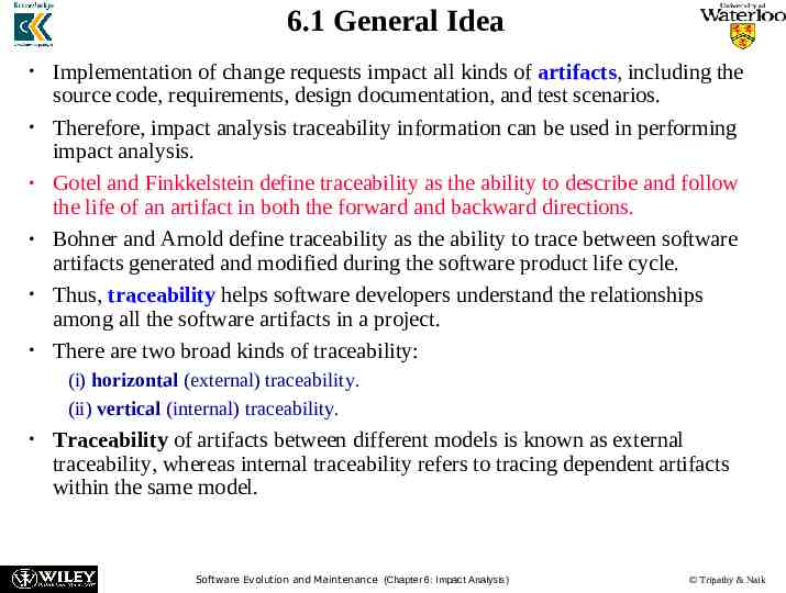
6.1 General Idea Implementation of change requests impact all kinds of artifacts, including the source code, requirements, design documentation, and test scenarios. Therefore, impact analysis traceability information can be used in performing impact analysis. Gotel and Finkkelstein define traceability as the ability to describe and follow the life of an artifact in both the forward and backward directions. Bohner and Arnold define traceability as the ability to trace between software artifacts generated and modified during the software product life cycle. Thus, traceability helps software developers understand the relationships among all the software artifacts in a project. There are two broad kinds of traceability: (i) horizontal (external) traceability. (ii) vertical (internal) traceability. Traceability of artifacts between different models is known as external traceability, whereas internal traceability refers to tracing dependent artifacts within the same model. Software Evolution and Maintenance (Chapter 6: Impact Analysis) Tripathy & Naik
6.1 General Idea A topic related to impact analysis is ripple effect analysis. Ripple effect means that a modification to a single variable may require several parts of the software system to be modified. Analysis of ripple effect reveals what and where changes are occurring. Measurement of ripple effects can provide the following information about an evolving software systems: (i) between successive versions of the same system, measurement of ripple effect will tell us how the software’s complexity has changed. (ii) when a new module is added to the system, measurement of ripple effect on the system will tell us how the software’s complexity has changed because of the addition of the new module. Software Evolution and Maintenance (Chapter 6: Impact Analysis) Tripathy & Naik
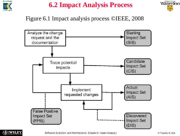
6.2 Impact Analysis Process Figure 6.1 Impact analysis process IEEE, 2008 Software Evolution and Maintenance (Chapter 6: Impact Analysis) Tripathy & Naik
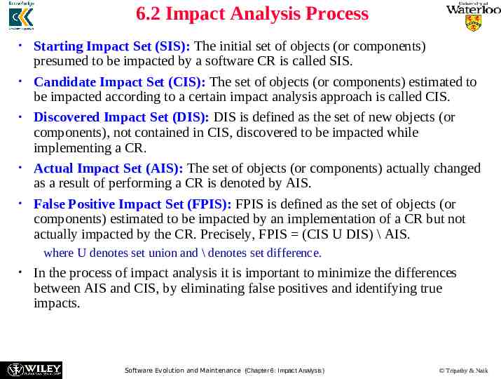
6.2 Impact Analysis Process Starting Impact Set (SIS): The initial set of objects (or components) presumed to be impacted by a software CR is called SIS. Candidate Impact Set (CIS): The set of objects (or components) estimated to be impacted according to a certain impact analysis approach is called CIS. Discovered Impact Set (DIS): DIS is defined as the set of new objects (or components), not contained in CIS, discovered to be impacted while implementing a CR. Actual Impact Set (AIS): The set of objects (or components) actually changed as a result of performing a CR is denoted by AIS. False Positive Impact Set (FPIS): FPIS is defined as the set of objects (or components) estimated to be impacted by an implementation of a CR but not actually impacted by the CR. Precisely, FPIS (CIS U DIS) \ AIS. where U denotes set union and \ denotes set difference. In the process of impact analysis it is important to minimize the differences between AIS and CIS, by eliminating false positives and identifying true impacts. Software Evolution and Maintenance (Chapter 6: Impact Analysis) Tripathy & Naik
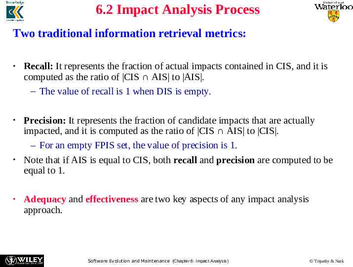
6.2 Impact Analysis Process Two traditional information retrieval metrics: Recall: It represents the fraction of actual impacts contained in CIS, and it is computed as the ratio of CIS AIS to AIS . – The value of recall is 1 when DIS is empty. Precision: It represents the fraction of candidate impacts that are actually impacted, and it is computed as the ratio of CIS AIS to CIS . – For an empty FPIS set, the value of precision is 1. Note that if AIS is equal to CIS, both recall and precision are computed to be equal to 1. Adequacy and effectiveness are two key aspects of any impact analysis approach. Software Evolution and Maintenance (Chapter 6: Impact Analysis) Tripathy & Naik
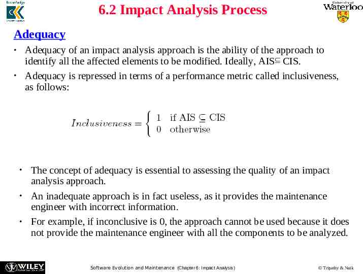
6.2 Impact Analysis Process Adequacy Adequacy of an impact analysis approach is the ability of the approach to identify all the affected elements to be modified. Ideally, AIS CIS. Adequacy is repressed in terms of a performance metric called inclusiveness, as follows: The concept of adequacy is essential to assessing the quality of an impact analysis approach. An inadequate approach is in fact useless, as it provides the maintenance engineer with incorrect information. For example, if inconclusive is 0, the approach cannot be used because it does not provide the maintenance engineer with all the components to be analyzed. Software Evolution and Maintenance (Chapter 6: Impact Analysis) Tripathy & Naik
6.2 Impact Analysis Process Effectiveness The ability of an impact analysis technique to generate results, that actually benefit the maintenance tasks, is known as its effectiveness. Effectiveness is expressed in terms of three fine grained characteristics as follows: – Ripple-sensitivity – Sharpness – Adherence Ripple-sensitivity Ripple-sensitivity implies producing results that are influenced by ripple effect. Software Evolution and Maintenance (Chapter 6: Impact Analysis) Tripathy & Naik
6.2 Impact Analysis Process Effectiveness Ripple-sensitivity The set of objects that are directly affected by the change is denoted by DISO (directly impacted set of objects). Similarly, the set of objects that are indirectly impacted by the change is denoted by IISO (indirectly impacted set of objects). The cardinality of IISO is an indicator of ripple effect. The software maintenance personnel expect that the cardinality of IISO is not far from the cardinality of DISO. Therefore, the concept of Amplification, as defined below, is used as a measure of Ripple-sensitivity. Amplification IISO / DISO 1; where . denotes the cardinality operator. Software Evolution and Maintenance (Chapter 6: Impact Analysis) Tripathy & Naik
6.2 Impact Analysis Process Effectiveness Sharpness Sharpness is the ability of an impact analysis approach to avoid having to include objects in the CIS that are not needed to be changed. Sharpness is expressed by means of Change Rate as defined below: ChangeRate CIS / System ChangeRate falls in the range from 0 to 1. Adherence Adherence is the ability of the approach to produce a CIS which is as close to AIS as possible. A small difference between CIS and AIS means that a small number of candidate objects fail to be included in the actual modification set. Adherence is expressed by S-Ratio as follows: S-Ratio AIS / CIS S-Ratio takes on values in the range from 0 to 1. Software Evolution and Maintenance (Chapter 6: Impact Analysis) Tripathy & Naik
6.2.1 Identifying the Starting Impact Set (SIS) Impact analysis begins with identifying the SIS. The CR specification, documentation, and source code are analyzed to find the SIS. It takes more efforts to map a new CR’s “concepts” onto source code components (or objects). In the “concept assignment problem,” one discovers human oriented concepts and assigns them to their realization. It is difficult to fully automate the concept assignment problem because programs and concepts do not occur at identical levels of abstractions, thereby necessitating human interactions. Software Evolution and Maintenance (Chapter 6: Impact Analysis) Tripathy & Naik
6.2.1 Identifying the Starting Impact Set (SIS) There are several methods to identify concepts, or features, in source code. The “grep” pattern matching utility available on most Unix systems and similar search tools are commonly used by programmers. However, the tool has some deficiencies: – it is based on the correspondence between the name for the concept assigned by the programmer and an identifier in the code. The technique often fails when the concepts are hidden in the source code, or when the programmer fails to guess the program identifiers. Software Evolution and Maintenance (Chapter 6: Impact Analysis) Tripathy & Naik
6.2.1 Identifying the Starting Impact Set (SIS) The software reconnaissance methodology proposed by Wilde and Scully is based on the idea that some programming concepts are selectable, because their execution depends on a specific input sequence. Selectable program concepts are known as features. By executing a program twice, one can often find the source code implementing the features: (i) execute the program once with a feature and once without the feature. (ii) mark portions of the source code that were executed the first time but not the second time. (iii) the marked code are likely to be in or close to the code implementing the feature. Software Evolution and Maintenance (Chapter 6: Impact Analysis) Tripathy & Naik
6.2.1 Identifying the Starting Impact Set (SIS) Chen and Rajlich proposed a dependency graph based feature location method for C programs. The component dependency graph is searched, generally beginning at the main(). Functions are chosen one at a time for a visit. The maintenance personnel reads the documentation, code, and dependency graph to comprehend the component before deciding if the component is related to the feature under consideration. Software Evolution and Maintenance (Chapter 6: Impact Analysis) Tripathy & Naik
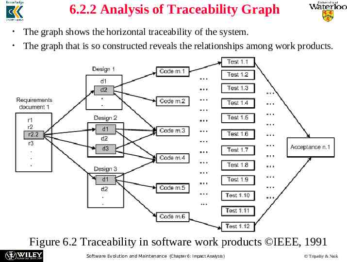
6.2.2 Analysis of Traceability Graph The graph shows the horizontal traceability of the system. The graph that is so constructed reveals the relationships among work products. Figure 6.2 Traceability in software work products IEEE, 1991 Software Evolution and Maintenance (Chapter 6: Impact Analysis) Tripathy & Naik
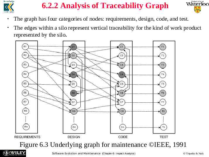
6.2.2 Analysis of Traceability Graph The graph has four categories of nodes: requirements, design, code, and test. The edges within a silo represent vertical traceability for the kind of work product represented by the silo. Figure 6.3 Underlying graph for maintenance IEEE, 1991 Software Evolution and Maintenance (Chapter 6: Impact Analysis) Tripathy & Naik
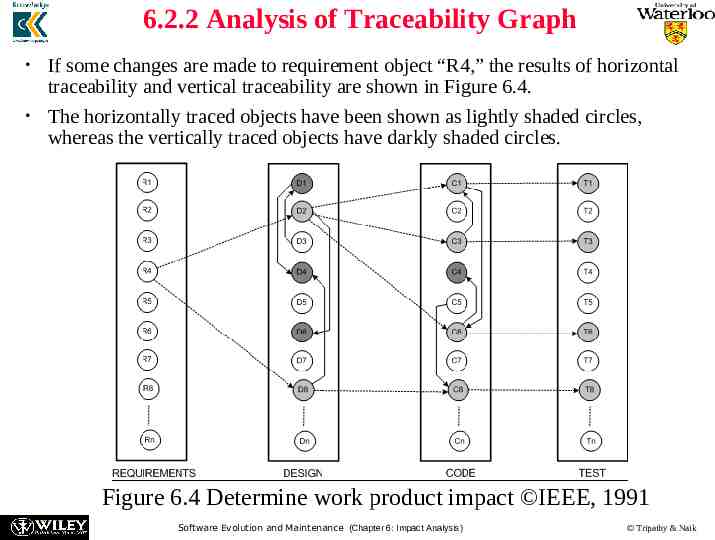
6.2.2 Analysis of Traceability Graph If some changes are made to requirement object “R4,” the results of horizontal traceability and vertical traceability are shown in Figure 6.4. The horizontally traced objects have been shown as lightly shaded circles, whereas the vertically traced objects have darkly shaded circles. Figure 6.4 Determine work product impact IEEE, 1991 Software Evolution and Maintenance (Chapter 6: Impact Analysis) Tripathy & Naik
6.2.2 Analysis of Traceability Graph For a node i in a graph, its in-degree in(i) counts the number of edges for which i is the destination node, and in(i) denotes the number of nodes having a direct impact on i. Similarly, the out-degree of node i, denoted by out(i), is the number of edges for which i is the source. Node i being changed, out(i) is a measure of the number of nodes which are likely to be modified. A common measure of complexity of a graph is the well-known Cyclomatic complexity. Software Evolution and Maintenance (Chapter 6: Impact Analysis) Tripathy & Naik
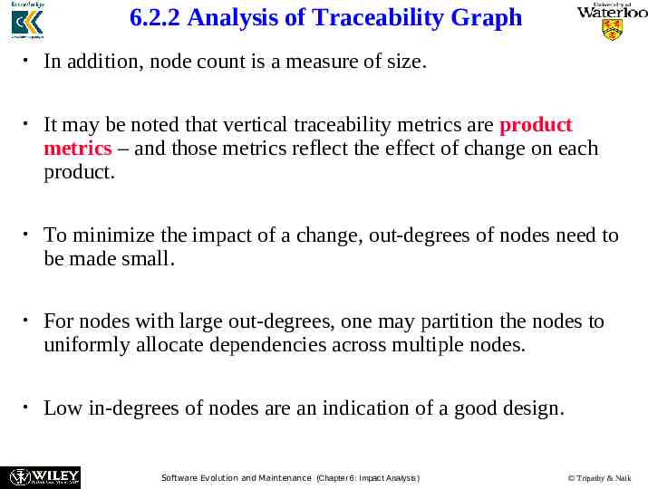
6.2.2 Analysis of Traceability Graph In addition, node count is a measure of size. It may be noted that vertical traceability metrics are product metrics – and those metrics reflect the effect of change on each product. To minimize the impact of a change, out-degrees of nodes need to be made small. For nodes with large out-degrees, one may partition the nodes to uniformly allocate dependencies across multiple nodes. Low in-degrees of nodes are an indication of a good design. Software Evolution and Maintenance (Chapter 6: Impact Analysis) Tripathy & Naik
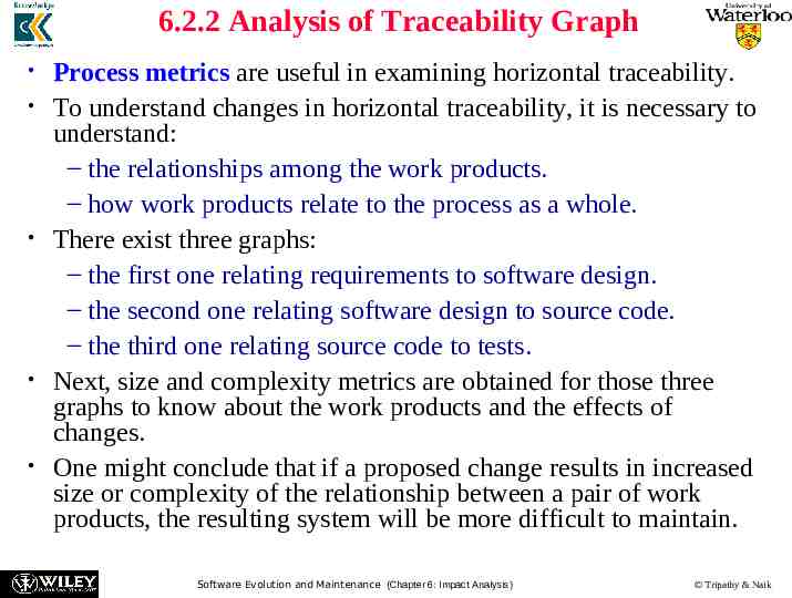
6.2.2 Analysis of Traceability Graph Process metrics are useful in examining horizontal traceability. To understand changes in horizontal traceability, it is necessary to understand: – the relationships among the work products. – how work products relate to the process as a whole. There exist three graphs: – the first one relating requirements to software design. – the second one relating software design to source code. – the third one relating source code to tests. Next, size and complexity metrics are obtained for those three graphs to know about the work products and the effects of changes. One might conclude that if a proposed change results in increased size or complexity of the relationship between a pair of work products, the resulting system will be more difficult to maintain. Software Evolution and Maintenance (Chapter 6: Impact Analysis) Tripathy & Naik
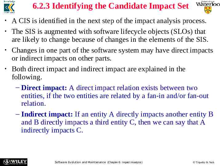
6.2.3 Identifying the Candidate Impact Set A CIS is identified in the next step of the impact analysis process. The SIS is augmented with software lifecycle objects (SLOs) that are likely to change because of changes in the elements of the SIS. Changes in one part of the software system may have direct impacts or indirect impacts on other parts. Both direct impact and indirect impact are explained in the following. – Direct impact: A direct impact relation exists between two entities, if the two entities are related by a fan-in and/or fan-out relation. – Indirect impact: If an entity A directly impacts another entity B and B directly impacts a third entity C, then we can say that A indirectly impacts C. Software Evolution and Maintenance (Chapter 6: Impact Analysis) Tripathy & Naik
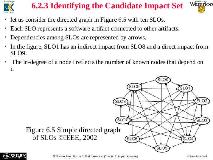
6.2.3 Identifying the Candidate Impact Set let us consider the directed graph in Figure 6.5 with ten SLOs. Each SLO represents a software artifact connected to other artifacts. Dependencies among SLOs are represented by arrows. In the figure, SLO1 has an indirect impact from SLO8 and a direct impact from SLO9. The in-degree of a node i reflects the number of known nodes that depend on i. Figure 6.5 Simple directed graph of SLOs IEEE, 2002 Software Evolution and Maintenance (Chapter 6: Impact Analysis) Tripathy & Naik
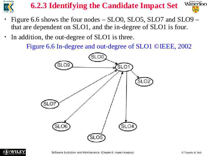
6.2.3 Identifying the Candidate Impact Set Figure 6.6 shows the four nodes – SLO0, SLO5, SLO7 and SLO9 – that are dependent on SLO1, and the in-degree of SLO1 is four. In addition, the out-degree of SLO1 is three. Figure 6.6 In-degree and out-degree of SLO1 IEEE, 2002 Software Evolution and Maintenance (Chapter 6: Impact Analysis) Tripathy & Naik
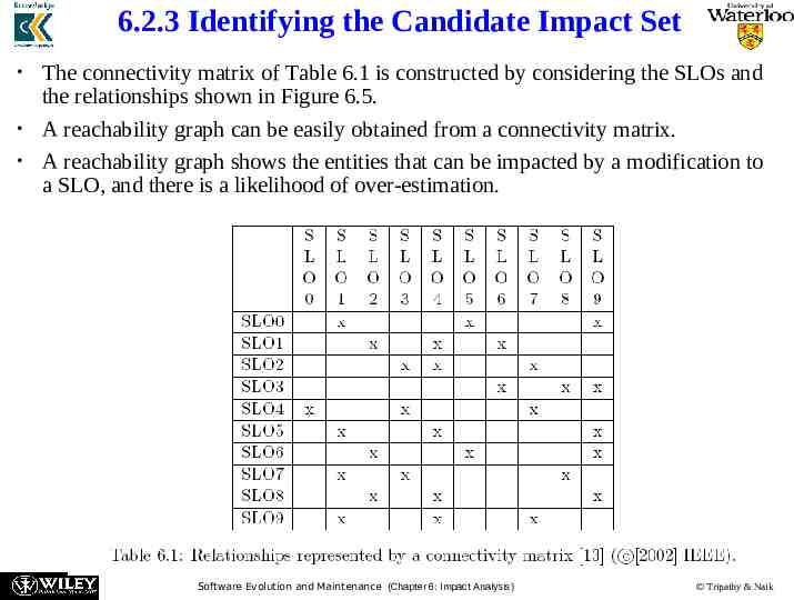
6.2.3 Identifying the Candidate Impact Set The connectivity matrix of Table 6.1 is constructed by considering the SLOs and the relationships shown in Figure 6.5. A reachability graph can be easily obtained from a connectivity matrix. A reachability graph shows the entities that can be impacted by a modification to a SLO, and there is a likelihood of over-estimation. Software Evolution and Maintenance (Chapter 6: Impact Analysis) Tripathy & Naik
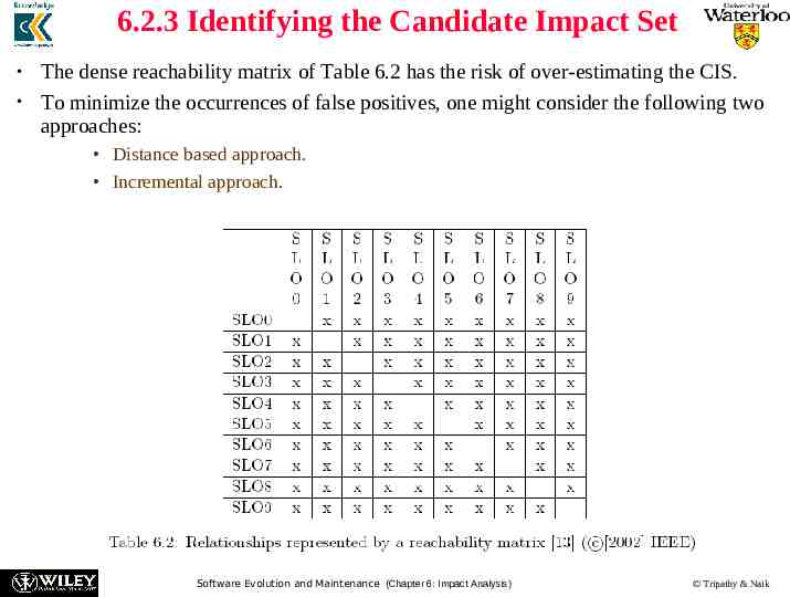
6.2.3 Identifying the Candidate Impact Set The dense reachability matrix of Table 6.2 has the risk of over-estimating the CIS. To minimize the occurrences of false positives, one might consider the following two approaches: Distance based approach. Incremental approach. Software Evolution and Maintenance (Chapter 6: Impact Analysis) Tripathy & Naik
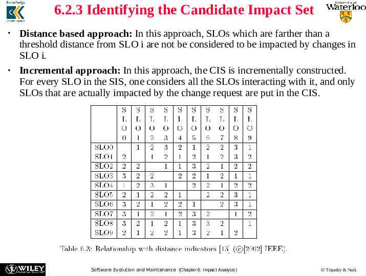
6.2.3 Identifying the Candidate Impact Set Distance based approach: In this approach, SLOs which are farther than a threshold distance from SLO i are not be considered to be impacted by changes in SLO i. Incremental approach: In this approach, the CIS is incrementally constructed. For every SLO in the SIS, one considers all the SLOs interacting with it, and only SLOs that are actually impacted by the change request are put in the CIS. Software Evolution and Maintenance (Chapter 6: Impact Analysis) Tripathy & Naik
6.3 Dependency-based Impact Analysis In general, source code objects are analyzed to obtain vertical traceability information. Dependency based impact analysis techniques identify the impact of changes by analyzing syntactic dependencies, because syntactic dependencies are likely to cause semantic dependencies. Two traditional impact analysis techniques are explained: – The first technique is based on call graph. – the second one is based on dependency graph. Software Evolution and Maintenance (Chapter 6: Impact Analysis) Tripathy & Naik
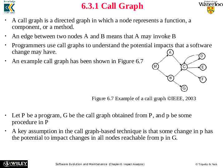
6.3.1 Call Graph A call graph is a directed graph in which a node represents a function, a component, or a method. An edge between two nodes A and B means that A may invoke B Programmers use call graphs to understand the potential impacts that a software change may have. An example call graph has been shown in Figure 6.7 Figure 6.7 Example of a call graph IEEE, 2003 Let P be a program, G be the call graph obtained from P, and p be some procedure in P A key assumption in the call graph-based technique is that some change in p has the potential to impact changes in all nodes reachable from p in G. Software Evolution and Maintenance (Chapter 6: Impact Analysis) Tripathy & Naik
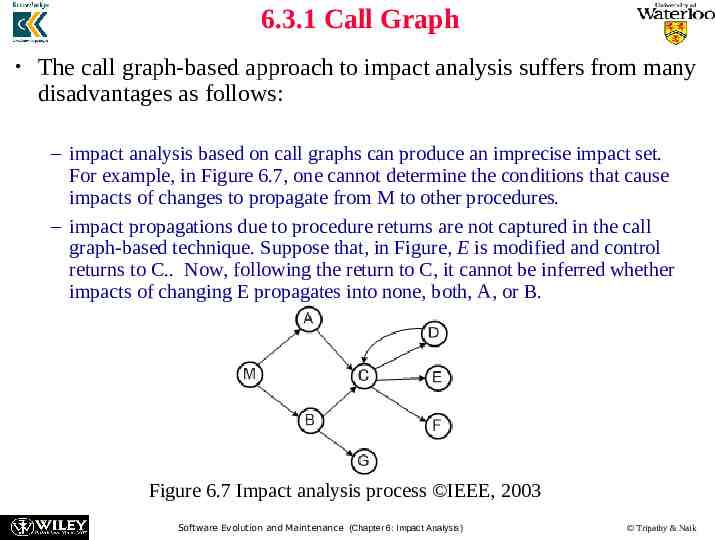
6.3.1 Call Graph The call graph-based approach to impact analysis suffers from many disadvantages as follows: – impact analysis based on call graphs can produce an imprecise impact set. For example, in Figure 6.7, one cannot determine the conditions that cause impacts of changes to propagate from M to other procedures. – impact propagations due to procedure returns are not captured in the call graph-based technique. Suppose that, in Figure, E is modified and control returns to C. Now, following the return to C, it cannot be inferred whether impacts of changing E propagates into none, both, A, or B. Figure 6.7 Impact analysis process IEEE, 2003 Software Evolution and Maintenance (Chapter 6: Impact Analysis) Tripathy & Naik
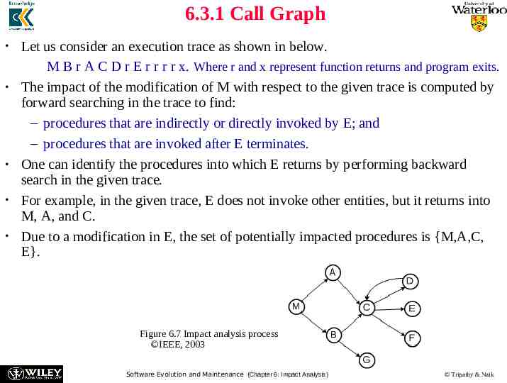
6.3.1 Call Graph Let us consider an execution trace as shown in below. M B r A C D r E r r r r x. Where r and x represent function returns and program exits. The impact of the modification of M with respect to the given trace is computed by forward searching in the trace to find: – procedures that are indirectly or directly invoked by E; and – procedures that are invoked after E terminates. One can identify the procedures into which E returns by performing backward search in the given trace. For example, in the given trace, E does not invoke other entities, but it returns into M, A, and C. Due to a modification in E, the set of potentially impacted procedures is {M,A,C, E}. Figure 6.7 Impact analysis process IEEE, 2003 Software Evolution and Maintenance (Chapter 6: Impact Analysis) Tripathy & Naik
6.3.2 Program Dependency Graph In the program dependency graph (PDG) of a program: (i) each simple statement is represented by a node, also called a vertex; (ii) each predicate expression is represented by a node. There are two types of edges in a PDG: data dependency edges and control dependency edges. Let vi and vj be two nodes in a PDG. If there is a data dependency edge from node vi to node vj , then the computations performed at node vi are directly dependent upon the results of computations performed at node vj . A control dependency edge from node vi to node vj indicates that node vi may execute based on the result of evaluation of a condition at vj . Software Evolution and Maintenance (Chapter 6: Impact Analysis) Tripathy & Naik
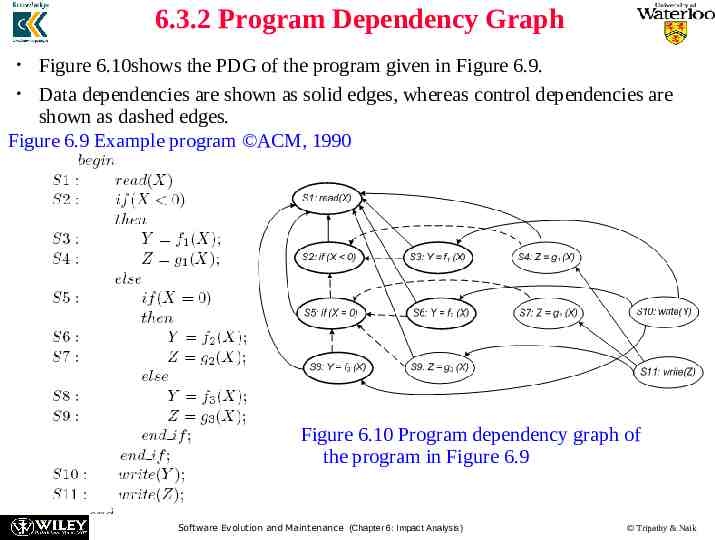
6.3.2 Program Dependency Graph Figure 6.10shows the PDG of the program given in Figure 6.9. Data dependencies are shown as solid edges, whereas control dependencies are shown as dashed edges. Figure 6.9 Example program ACM, 1990 Figure 6.10 Program dependency graph of the program in Figure 6.9 Software Evolution and Maintenance (Chapter 6: Impact Analysis) Tripathy & Naik
6.3.2 Program Dependency Graph Static Program Slice A static program slice is identified from a PDG as follows: for a variable var at node n, identify all reaching definitions of var. find all nodes in the PDG which are reachable from those nodes. The visited nodes in the traversal process constitute the desired slice. Consider the program in the previous slide and variable Y at S10. First, find all the reaching definitions of Y at node S10 – and the answer is the set of nodes {S3, S6 and S8}. Next, find the set of all nodes which are reachable from {S3, S6 and S8} – and the answer is the set {S1, S2, S3, S5, S6, S8}. In the program dependency graph the nodes belonging in the slice have been identified in bold. Software Evolution and Maintenance (Chapter 6: Impact Analysis) Tripathy & Naik
6.3.2 Program Dependency Graph Dynamic Slice A dynamic slice is more useful in localizing the defect than the static slice. Only one of the three assignment statements, S3, S6, or S8, may be executed for any input value of X. Consider the input value 1 for the variable X. For 1 as the value of X, only S3 is executed. Therefore, with respect to variable Y at S10, the dynamic slice will contain only {S1, S2 and S3}. Software Evolution and Maintenance (Chapter 6: Impact Analysis) Tripathy & Naik
6.3.2 Program Dependency Graph Dynamic Slice For 1 as the values of X, if the value of Y is incorrect at S10, one can infer that either fi is erroneous at S3 or the “if” condition at S2 is incorrect. A simple approach to obtaining dynamic program slices is explained here. Given a test and a PDG, let us represent the execution history of the program as a sequence of vertices v1, v2, ., vn . The execution history hist of a program P for a test case test, and a variable var is the set of all statements in hist whose execution had some effect on the value of var as observed at the end of the execution. Software Evolution and Maintenance (Chapter 6: Impact Analysis) Tripathy & Naik
6.3.2 Program Dependency Graph Dynamic Slice Now, in our example discussed before, the static program slice with respect to variable Y at S10 for the code contains all the three statements – S3, S6, and S8. However, for a given test, one statement from the set {S3, S6, and S8} is executed. A simple way to finding dynamic slices is as follows: (i) for the current test, mark the executed nodes in the PDG. (ii) traverse the marked nodes in the graph. Software Evolution and Maintenance (Chapter 6: Impact Analysis) Tripathy & Naik
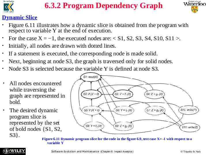
6.3.2 Program Dependency Graph Dynamic Slice Figure 6.11 illustrates how a dynamic slice is obtained from the program with respect to variable Y at the end of execution. For the case X 1, the executed nodes are: S1, S2, S3, S4, S10, S11 . Initially, all nodes are drawn with dotted lines. If a statement is executed, the corresponding node is made solid. Next, beginning at node S3, the graph is traversed only for solid nodes. Node S3 is selected because the variable Y is defined at node S3. All nodes encountered while traversing the graph are represented in bold. The desired dynamic program slice is represented by the set of bold nodes {S1, S2, S3}. Figure 6.11 Dynamic program slice for the code in the figure 6.9, test case X -1 with respect to a variable Y Software Evolution and Maintenance (Chapter 6: Impact Analysis) Tripathy & Naik
6.4 Ripple Effect Haney introduced the concept of ripple effect in the early 1970s. From the functional and performance perspectives, Yau, Collofello and McGregor defined the concept of ripple effect in 1978. They viewed ripple effect as a complexity measure to compare changes to source code. In the scheme of Yau et al., ripple effect is computed by means of error flow analysis. In error flow analysis, definitions of program variables involved in a change are considered to be potential sources of errors. Software Evolution and Maintenance (Chapter 6: Impact Analysis) Tripathy & Naik
6.4 Ripple Effect Inconsistency can propagate from those sources to other variables in the program. The other sources of errors are successively identified until error propagation is no more possible. This work was later extended to include stability measure. Stability reflects the resistance to the potential ripple effect which a program would have when it is changed. Stability analysis and impact analysis differ as follows: – stability analysis considers the total potential ripple effects rather than a specific ripple effect caused by a change. Software Evolution and Maintenance (Chapter 6: Impact Analysis) Tripathy & Naik
6.4 Ripple Effect Design stability was studied by Yau and Collofello by means of an algorithm, which computes stability based on design documentation. Specifically, one counts the number of assumptions made about shared global data structures and module interfaces. The key difference between design level stability and code level stability is as follows: Design level stability does not consider change propagations within modules. Next we explain how to compute ripple effect, based on the works of Sue Black. The basic idea is to identify the impact of a change to one variable on the program. Software Evolution and Maintenance (Chapter 6: Impact Analysis) Tripathy & Naik
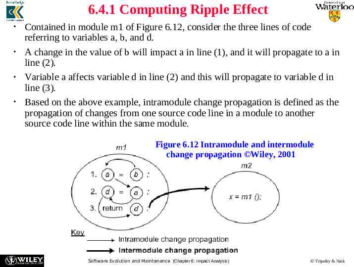
6.4.1 Computing Ripple Effect Contained in module m1 of Figure 6.12, consider the three lines of code referring to variables a, b, and d. A change in the value of b will impact a in line (1), and it will propagate to a in line (2). Variable a affects variable d in line (2) and this will propagate to variable d in line (3). Based on the above example, intramodule change propagation is defined as the propagation of changes from one source code line in a module to another source code line within the same module. Figure 6.12 Intramodule and intermodule change propagation Wiley, 2001 Software Evolution and Maintenance (Chapter 6: Impact Analysis) Tripathy & Naik
6.4.1 Computing Ripple Effect Propagation of values of variables in one module to variables in a different module is referred to as intermodule change propagation. Intermodule change propagation of values of a variable w occurs in the following ways: – If w is a global variable, then a change made to w by one module is seen by another module accessing w. – If w is an input parameter in a call to a second module, then values of w are propagated from the caller to the callee. – If w is an output parameter, then its value propagates from the module that makes an output to the module that accepts the output. Now we examine the code segment in Figure 6.12. Variable d propagates to any module that calls m1, because d appears in the return statement. If variable a is global, its appearance on the left-hand-side of an assignment statement causes its value to be propagated to any module that uses variable a. Software Evolution and Maintenance (Chapter 6: Impact Analysis) Tripathy & Naik
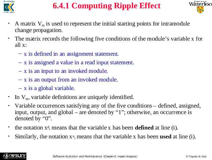
6.4.1 Computing Ripple Effect A matrix Vm is used to represent the initial starting points for intramodule change propagation. The matrix records the following five conditions of the module’s variable x for all x: – x is defined in an assignment statement. – x is assigned a value in a read input statement. – x is an input to an invoked module. – x is an output from an invoked module. – x is a global variable. In Vm, variable definitions are uniquely identified. Variable occurrences satisfying any of the five conditions – defined, assigned, input, output, and global – are denoted by “1”; otherwise, an occurrence is denoted by “0”. the notation xdi means that the variable x has been defined at line (i). Similarly, the notation xui means that the variable x has been used at line (i). Software Evolution and Maintenance (Chapter 6: Impact Analysis) Tripathy & Naik
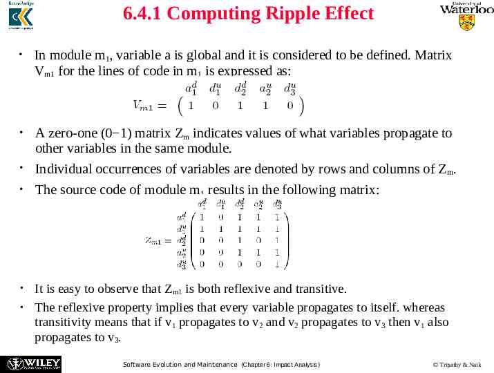
6.4.1 Computing Ripple Effect In module m1, variable a is global and it is considered to be defined. Matrix Vm1 for the lines of code in m1 is expressed as: A zero-one (0 1) matrix Zm indicates values of what variables propagate to other variables in the same module. Individual occurrences of variables are denoted by rows and columns of Z m. The source code of module m1 results in the following matrix: It is easy to observe that Zm1 is both reflexive and transitive. The reflexive property implies that every variable propagates to itself. whereas transitivity means that if v1 propagates to v2 and v2 propagates to v3 then v1 also propagates to v3. Software Evolution and Maintenance (Chapter 6: Impact Analysis) Tripathy & Naik
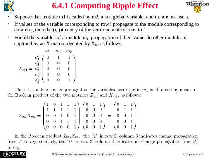
6.4.1 Computing Ripple Effect Suppose that module m1 is called by m2, a is a global variable, and m 2 and m3 use a. If values of the variable corresponding to row i propagate to the module corresponding to column j, then the (i, j)th entry of the zero-one matrix is set to 1. For all the variables of a module m1, propagation of their values to other modules is captured by an X matrix, denoted by Xm1 as follows: Software Evolution and Maintenance (Chapter 6: Impact Analysis) Tripathy & Naik
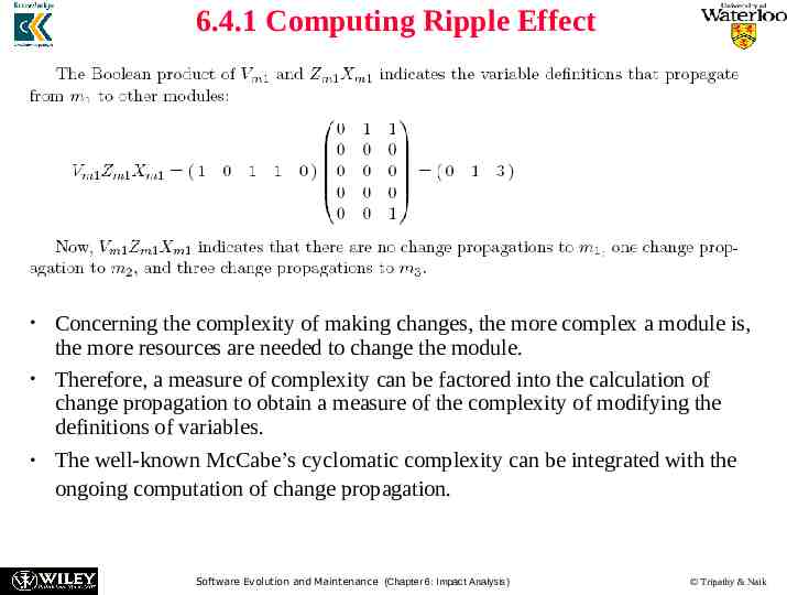
6.4.1 Computing Ripple Effect Concerning the complexity of making changes, the more complex a module is, the more resources are needed to change the module. Therefore, a measure of complexity can be factored into the calculation of change propagation to obtain a measure of the complexity of modifying the definitions of variables. The well-known McCabe’s cyclomatic complexity can be integrated with the ongoing computation of change propagation. Software Evolution and Maintenance (Chapter 6: Impact Analysis) Tripathy & Naik
6.4.1 Computing Ripple Effect A C matrix of dimensions 1 n is chosen to represent McCabe’s cyclomatic complexity, where n is the number of modules: Software Evolution and Maintenance (Chapter 6: Impact Analysis) Tripathy & Naik
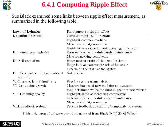
6.4.1 Computing Ripple Effect Sue Black examined some links between ripple effect measurement, as summarized in the following table. Software Evolution and Maintenance (Chapter 6: Impact Analysis) Tripathy & Naik
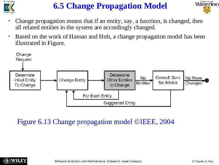
6.5 Change Propagation Model Change propagation means that if an entity, say, a function, is changed, then all related entities in the system are accordingly changed. Based on the work of Hassan and Holt, a change propagation model has been illustrated in Figure. Figure 6.13 Change propagation model IEEE, 2004 Software Evolution and Maintenance (Chapter 6: Impact Analysis) Tripathy & Naik
6.5.1 Recall and Precision of Change Propagation Heuristics Gurus rarely exist and comprehensive test suites are generally incomplete in large maintenance projects. Therefore, software maintenance engineers need good change propagation heuristics, that is, good software tools that can guide them in identifying entities to propagate a change. The heuristic should possess the high precision attribute to be accurate and the high recall attribute to be complete. We explained the concepts of recall and precision before. Next, we explain the use of those two metrics to measure the change propagation heuristic by means of an example. Software Evolution and Maintenance (Chapter 6: Impact Analysis) Tripathy & Naik
6.5.1 Recall and Precision of Change Propagation Heuristics Example: Let us assume that Rohan wants to enhance an existing feature of a legacy information system. He first identifies that entity A needs to be changed. After changing A, an heuristic tool is queried for suggestions, and entities B and X are suggested by the tool. Next, B is changed and he determines that X should not be changed. Now the tool is given the information that B was changed, and the tool suggests that Y and W need to be changed. However, neither Y nor W need to be changed so no changes are performed on Y and W. After having used the tool, now Rohan consults a Guru, Krushna. Krushna indicates that C should be changed. Now, Rohan modifies C and queries the heuristic for additional entities to change. In response, D is suggested by the tool. Next, D is changed and Krushna is further queried. However, this time Krushna does not suggest any more entities for change. Now, Rohan stops changing the legacy system. Software Evolution and Maintenance (Chapter 6: Impact Analysis) Tripathy & Naik
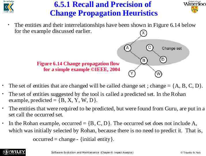
6.5.1 Recall and Precision of Change Propagation Heuristics The entities and their interrelationships have been shown in Figure 6.14 below for the example discussed earlier. Figure 6.14 Change propagation flow for a simple example IEEE, 2004 The set of entities that are changed will be called change set ; change {A, B, C, D}. The set of entities suggested by the tool is called a predicted set. In the Rohan example, predicted {B, X, Y, W, D}. The entities that were required to be predicted, but were found from Guru, are put in a set call the occurred set. In the Rohan example, occurred {B, C, D}. The occurred set does not include A, which was initially selected by Rohan, because there is no need to predict it. That is, occurred change - {initial entity}. Software Evolution and Maintenance (Chapter 6: Impact Analysis) Tripathy & Naik
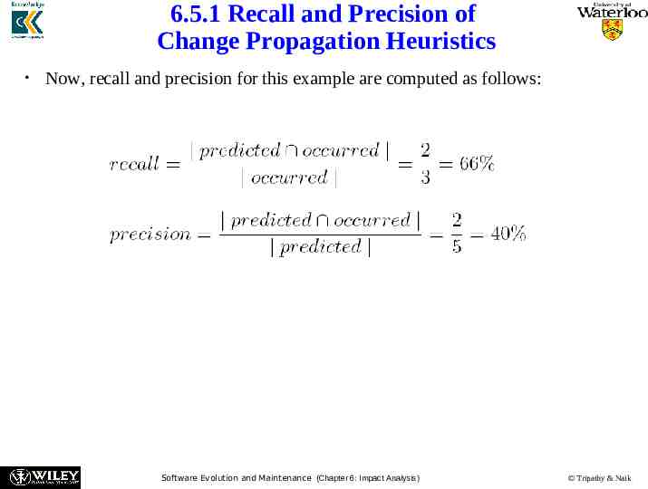
6.5.1 Recall and Precision of Change Propagation Heuristics Now, recall and precision for this example are computed as follows: Software Evolution and Maintenance (Chapter 6: Impact Analysis) Tripathy & Naik
6.5.1 Recall and Precision of Change Propagation Heuristics In the analysis of the example is to measure recall and precision the authors, Hassan and Holt, made three assumptions: 1. Symmetric suggestions: This assumption means that if the tool suggests entity F to be modified when it is told that entity E was changed, the tool will suggest entity E to be modified when it is told that entity F was changed. This assumption has been depicted in Figure by means of undirected edges. 2. Single entity suggestions: This assumption means that each prediction by a heuristic tool is performed by considering a single entity known to be in the change set, rather than multiple entities in the change set. 3. Query the tool first: This assumption means that the maintainer (e.g., Rohan) will query the heuristic before doing so with the Guru (e.g. Krushna). Software Evolution and Maintenance (Chapter 6: Impact Analysis) Tripathy & Naik
6.5.2 Heuristics for Change Propagation The “Determine Other Entities to Change” step in Figure 6.13 is executed by means of several heuristics. The set of entities that need to be changed as a result of a changed entity is computed in the aforementioned step. Modification records are central to the design of the heuristics. In general, source control repositories are used to keep track of all the changes made to files in the system. Each heuristic discussed here is characterized by: (i) data source. (ii) pruning technique. Software Evolution and Maintenance (Chapter 6: Impact Analysis) Tripathy & Naik
6.5.2 Heuristics for Change Propagation Heuristic Information Sources The objectives of the heuristics are to: (i) ensure that the entities that need to be modified are predicted. (ii) minimize the number of predicted entities that are not going to be modified. Some potential information sources are as follows: – – – – Entity information Developer information (DEV) Process information Textual information Software Evolution and Maintenance (Chapter 6: Impact Analysis) Tripathy & Naik
6.5.2 Heuristics for Change Propagation Entity information In an heuristic based on entity information, a change propagates to other entities as follows: – If two entities changed together, then the two are called a historical cochange (HIS). – Static dependencies between two entities may occur via what is called CUD relations: call, use and define. A call relation means one function calls another function; a use relation means a variable is used by a function; and a define relation means a variable is defined in a function or it appears as a parameter in the function. – The locations of entities with respect to subsystems, files, and classes in the source code are represented by means of a code layout (FIL) relation. Subsystems, files, and classes indicate relations between entities – and, generally, related entities simultaneously. Software Evolution and Maintenance (Chapter 6: Impact Analysis) Tripathy & Naik
6.5.2 Heuristics for Change Propagation Developer information (DEV) In an heuristic based on developer information, a change propagates to other entities changed by the same developer. In general, programmers develop skills in specific subject matters of the system and it is more likely that they modify entities within their field of expertise. Process information In an heuristic based on process information, change propagation depends on the development process followed. A modification to a specific entity generally causes modifications to other recently or frequently changed entities. Textual information In an heuristic based on name similarity, changes are propagated to entities with similar names. Naming similarities indicate that there are similarities in the role of the entities. Software Evolution and Maintenance (Chapter 6: Impact Analysis) Tripathy & Naik
6.5.2 Heuristics for Change Propagation Pruning Techniques A heuristic may suggest a large number of entities to be changed. Several techniques can be applied to reduce the size of the suggested set, and those are called pruning techniques. Frequency techniques identify the frequently changing, related components. The number of entities returned by these techniques are constrained by a threshold. Recency techniques identify entities that were recently changed, thereby supporting the intuition that modifications generally focus on related code and functionality in a particular time frame. Random techniques randomly choose a set of entities, up to a threshold. In the absence of no frequency or recency data, one may use this technique. Software Evolution and Maintenance (Chapter 6: Impact Analysis) Tripathy & Naik
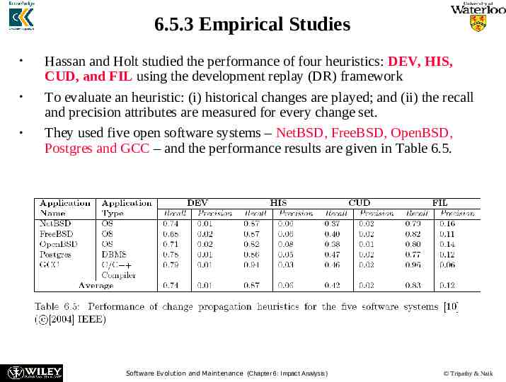
6.5.3 Empirical Studies Hassan and Holt studied the performance of four heuristics: DEV, HIS, CUD, and FIL using the development replay (DR) framework To evaluate an heuristic: (i) historical changes are played; and (ii) the recall and precision attributes are measured for every change set. They used five open software systems – NetBSD, FreeBSD, OpenBSD, Postgres and GCC – and the performance results are given in Table 6.5. Software Evolution and Maintenance (Chapter 6: Impact Analysis) Tripathy & Naik
Summary General Idea Impact Analysis Process Dependency-based Impact Analysis Ripple Effect Change Propagation Model Software Evolution and Maintenance (Chapter 6: Impact Analysis) Tripathy & Naik