Primer on Cash Flow Valuation

37 Slides612.00 KB
Primer on Cash Flow Valuation
The greater danger for most of us is not that our aim is too high and we might miss it, but that it is too low and we reach it. —Michelangelo
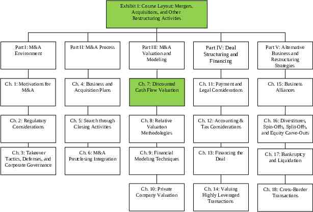
Exhibit 1: Course Layout: Mergers, Acquisitions, and Other Restructuring Activities Part I: M&A Environment Part II: M&A Process Part III: M&A Valuation and Modeling Part IV: Deal Structuring and Financing Part V: Alternative Business and Restructuring Strategies Ch. 1: Motivations for M&A Ch. 4: Business and Acquisition Plans Ch. 7: Discounted Cash Flow Valuation Ch. 11: Payment and Legal Considerations Ch. 15: Business Alliances Ch. 2: Regulatory Considerations Ch. 5: Search through Closing Activities Ch. 8: Relative Valuation Methodologies Ch. 12: Accounting & Tax Considerations Ch. 16: Divestitures, Spin-Offs, Split-Offs, and Equity Carve-Outs Ch. 3: Takeover Tactics, Defenses, and Corporate Governance Ch. 6: M&A Postclosing Integration Ch. 9: Financial Modeling Techniques Ch. 13: Financing the Deal Ch. 17: Bankruptcy and Liquidation Ch. 10: Private Company Valuation Ch. 14: Valuing Highly Leveraged Transactions Ch. 18: Cross-Border Transactions
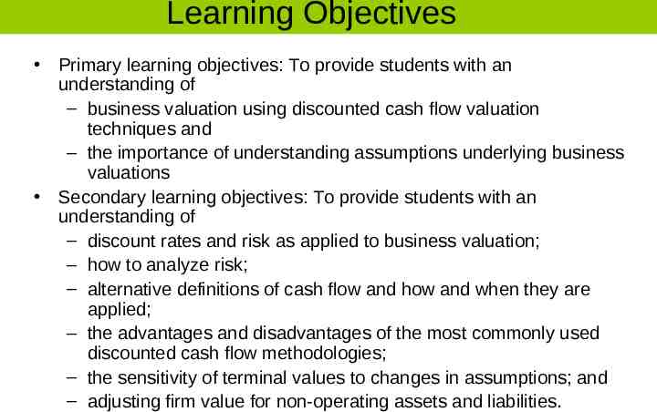
Learning Objectives Primary learning objectives: To provide students with an understanding of – business valuation using discounted cash flow valuation techniques and – the importance of understanding assumptions underlying business valuations Secondary learning objectives: To provide students with an understanding of – discount rates and risk as applied to business valuation; – how to analyze risk; – alternative definitions of cash flow and how and when they are applied; – the advantages and disadvantages of the most commonly used discounted cash flow methodologies; – the sensitivity of terminal values to changes in assumptions; and – adjusting firm value for non-operating assets and liabilities.
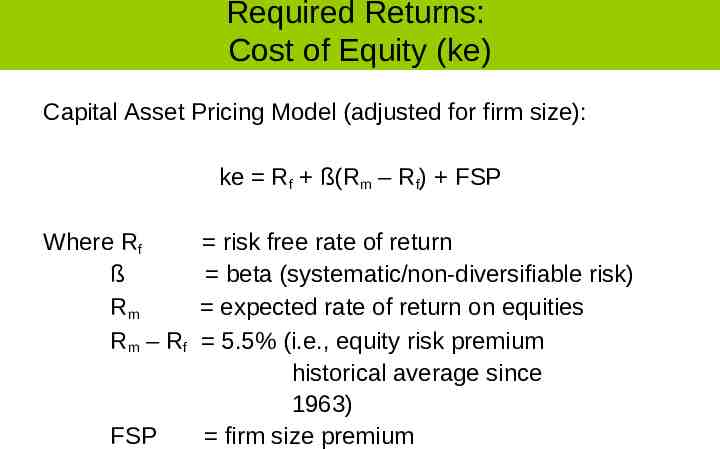
Required Returns: Cost of Equity (ke) Capital Asset Pricing Model (adjusted for firm size): ke Rf ß(Rm – Rf) FSP Where Rf ß Rm Rm – Rf FSP risk free rate of return beta (systematic/non-diversifiable risk) expected rate of return on equities 5.5% (i.e., equity risk premium historical average since 1963) firm size premium
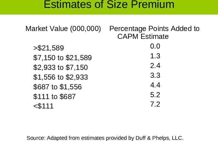
Estimates of Size Premium Market Value (000,000) 21,589 7,150 to 21,589 2,933 to 7,150 1,556 to 2,933 687 to 1,556 111 to 687 111 Percentage Points Added to CAPM Estimate 0.0 1.3 2.4 3.3 4.4 5.2 7.2 Source: Adapted from estimates provided by Duff & Phelps, LLC.
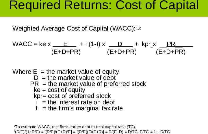
Required Returns: Cost of Capital Weighted Average Cost of Capital (WACC):1,2 WACC ke x E i (1-t) x D kpr x PR (E D PR) (E D PR) (E D PR) Where E the market value of equity D the market value of debt PR the market value of preferred stock ke cost of equity kpr cost of preferred stock i the interest rate on debt t the firm’s marginal tax rate 1 2 To estimate WACC, use firm’s target debt-to-total capital ratio (TC). (D/E)/(1 D/E) [(D/E)/(E D)/E] [(D/E)(E/(E D)] D/(E D) D/TC; E/TC 1 – D/TC.
Analyzing Risk Risk consists of a non-systematic/diversifiable and systematic/non-diversifiable component Beta (ß) is a measure of non-diversifiable risk Beta quantifies a stock’s volatility relative to the overall market Beta is impacted by the following factors: – Degree of industry cyclicality – Operating leverage refers to the composition of a firm’s cost structure (fixed plus variable costs) – Financial leverage refers to the composition of a firm’s capital structure (debt equity) Firms with high ratios of fixed to total costs and debt to total capital tend to display highly volatility and betas
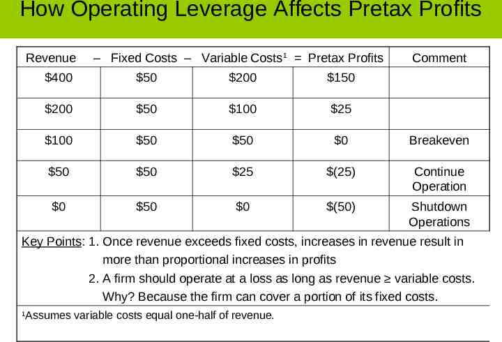
How Operating Leverage Affects Pretax Profits Revenue – Fixed Costs – Variable Costs1 Pretax Profits Comment 400 50 200 150 200 50 100 25 100 50 50 0 Breakeven 50 50 25 (25) Continue Operation 0 50 0 (50) Shutdown Operations Key Points: 1. Once revenue exceeds fixed costs, increases in revenue result in more than proportional increases in profits 2. A firm should operate at a loss as long as revenue variable costs. Why? Because the firm can cover a portion of its fixed costs. 1 Assumes variable costs equal one-half of revenue.
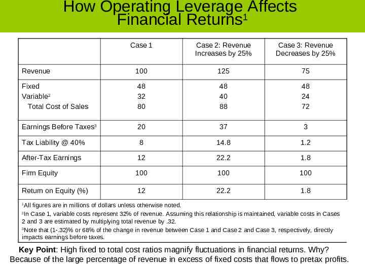
How Operating Leverage Affects Financial Returns1 Case 1 Case 2: Revenue Increases by 25% Case 3: Revenue Decreases by 25% Revenue 100 125 75 Fixed Variable2 Total Cost of Sales 48 32 80 48 40 88 48 24 72 Earnings Before Taxes3 20 37 3 Tax Liability @ 40% 8 14.8 1.2 After-Tax Earnings 12 22.2 1.8 Firm Equity 100 100 100 Return on Equity (%) 12 22.2 1.8 All figures are in millions of dollars unless otherwise noted. In Case 1, variable costs represent 32% of revenue. Assuming this relationship is maintained, variable costs in Cases 2 and 3 are estimated by multiplying total revenue by .32. 3 Note that (1-.32)% or 68% of the change in revenue between Case 1 and Case 2 and Case 3, respectively, directly impacts earnings before taxes. 1 2 Key Point: High fixed to total cost ratios magnify fluctuations in financial returns. Why? Because of the large percentage of revenue in excess of fixed costs that flows to pretax profits.
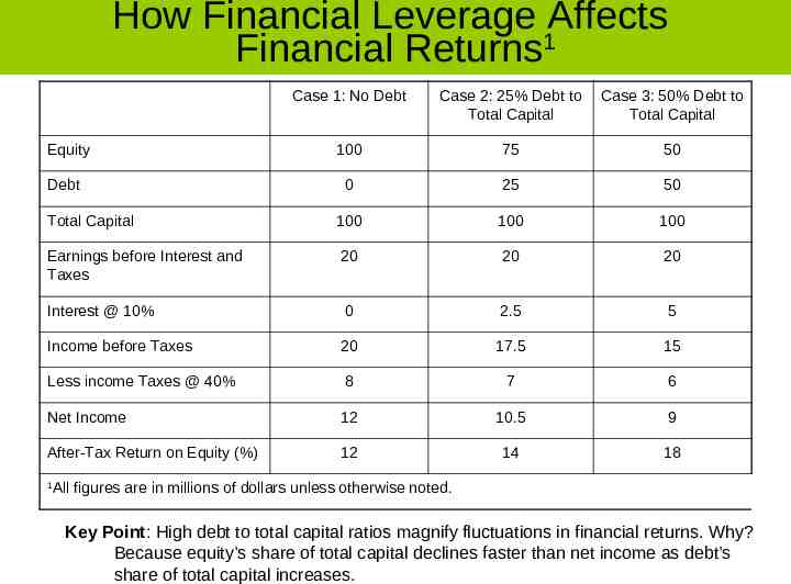
How Financial Leverage Affects Financial Returns1 Case 1: No Debt Case 2: 25% Debt to Total Capital Case 3: 50% Debt to Total Capital 100 75 50 0 25 50 Total Capital 100 100 100 Earnings before Interest and Taxes 20 20 20 Interest @ 10% 0 2.5 5 Income before Taxes 20 17.5 15 Less income Taxes @ 40% 8 7 6 Net Income 12 10.5 9 After-Tax Return on Equity (%) 12 14 18 Equity Debt 1 All figures are in millions of dollars unless otherwise noted. Key Point: High debt to total capital ratios magnify fluctuations in financial returns. Why? Because equity’s share of total capital declines faster than net income as debt’s share of total capital increases.
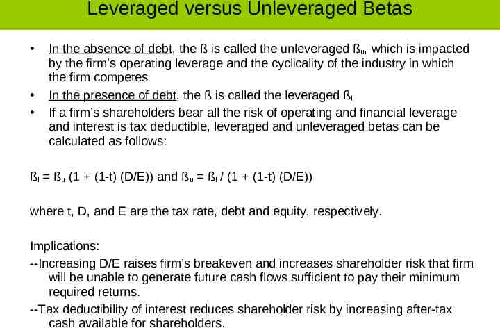
Leveraged versus Unleveraged Betas In the absence of debt, the ß is called the unleveraged ßu, which is impacted by the firm’s operating leverage and the cyclicality of the industry in which the firm competes In the presence of debt, the ß is called the leveraged ßl If a firm’s shareholders bear all the risk of operating and financial leverage and interest is tax deductible, leveraged and unleveraged betas can be calculated as follows: ßl ßu (1 (1-t) (D/E)) and ßu ßl / (1 (1-t) (D/E)) where t, D, and E are the tax rate, debt and equity, respectively. Implications: --Increasing D/E raises firm’s breakeven and increases shareholder risk that firm will be unable to generate future cash flows sufficient to pay their minimum required returns. --Tax deductibility of interest reduces shareholder risk by increasing after-tax cash available for shareholders.
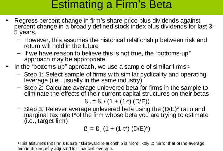
Estimating a Firm’s Beta Regress percent change in firm’s share price plus dividends against percent change in a broadly defined stock index plus dividends for last 35 years. – However, this assumes the historical relationship between risk and return will hold in the future – If we have reason to believe this is not true, the “bottoms-up” approach may be appropriate. In the “bottoms-up” approach, we use a sample of similar firms:1 – Step 1: Select sample of firms with similar cyclicality and operating leverage (i.e., usually in the same industry) – Step 2: Calculate average unlevered beta for firms in the sample to eliminate the effects of their current capital structures on their betas ßu ßl / (1 (1-t) (D/E)) – Step 3: Relever average unlevered beta using the (D/E)* ratio and marginal tax rate t*of the firm whose beta you are trying to estimate (i.e., target firm) ßl ßu (1 (1-t*) (D/E)*) This assumes the firm’s future risk/reward relationship is more likely to mirror that of the average firm in the industry adjusted for financial leverage. 1
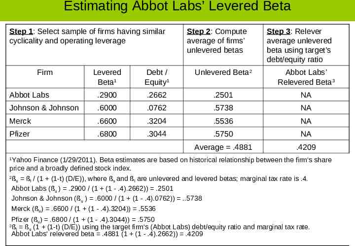
Estimating Abbot Labs’ Levered Beta Step 1: Select sample of firms having similar cyclicality and operating leverage Firm Step 2: Compute average of firms’ unlevered betas Step 3: Relever average unlevered beta using target’s debt/equity ratio Levered Beta1 Debt / Equity1 Unlevered Beta2 Abbot Labs’ Relevered Beta3 Abbot Labs .2900 .2662 .2501 NA Johnson & Johnson .6000 .0762 .5738 NA Merck .6600 .3204 .5536 NA Pfizer .6800 .3044 .5750 NA Average .4881 .4209 Yahoo Finance (1/29/2011). Beta estimates are based on historical relationship between the firm’s share price and a broadly defined stock index. 2 ßu ßl / (1 (1-t) (D/E)), where ßu and ßl are unlevered and levered betas; marginal tax rate is .4. Abbot Labs (ßu ) .2900 / (1 (1 - .4).2662)) .2501 Johnson & Johnson (ßu ) .6000 / (1 (1 - .4).0762)) .5738 Merck (ßu) .6600 / (1 (1 - .4).3204)) .5536 1 Pfizer (ßu) .6800 / (1 (1 - .4).3044)) .5750 ßl ßu (1 (1-t) (D/E)) using the target firm’s (Abbot Labs) debt/equity ratio and marginal tax rate. Abbot Labs’ relevered beta .4881 (1 (1 - .4).2662)) .4209 3
Valuation Cash Flow Valuation cash flows represent actual cash flows available to reward both shareholders and lenders Cash flow statements include cash inflows and outflows from: – operating, – investing, and – financing activities GAAP cash flows are adjusted for noncash inflows and outflows to calculate valuation cash flow. Examples include the following: – Adding depreciation back to net income – Deducting gains from and adding losses to net income resulting from asset sales Valuation cash flows include free cash flows to equity investors or equity cash flow and free cash flows to the firm or enterprise cash flow
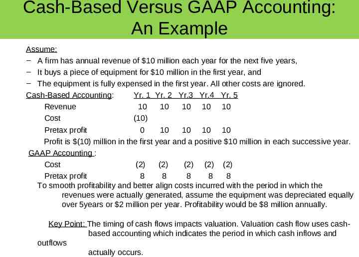
Cash-Based Versus GAAP Accounting: An Example Assume: – A firm has annual revenue of 10 million each year for the next five years, – It buys a piece of equipment for 10 million in the first year, and – The equipment is fully expensed in the first year. All other costs are ignored. Cash-Based Accounting: Yr. 1 Yr. 2 Yr.3 Yr.4 Yr. 5 Revenue 10 10 10 10 10 Cost (10) Pretax profit 0 10 10 10 10 Profit is (10) million in the first year and a positive 10 million in each successive year. GAAP Accounting : Cost (2) (2) (2) (2) (2) Pretax profit 8 8 8 8 8 To smooth profitability and better align costs incurred with the period in which the revenues were actually generated, assume the equipment was depreciated equally over 5years or 2 million per year. Profitability would be 8 million annually. Key Point: The timing of cash flows impacts valuation. Valuation cash flow uses cashbased accounting which indicates the period in which cash inflows and outflows actually occurs.
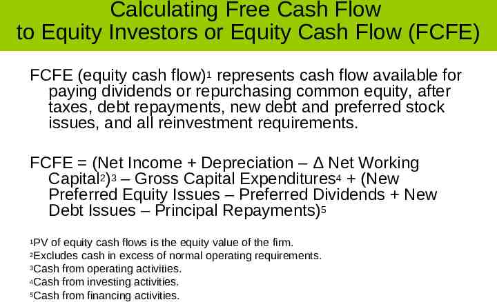
Calculating Free Cash Flow to Equity Investors or Equity Cash Flow (FCFE) FCFE (equity cash flow)1 represents cash flow available for paying dividends or repurchasing common equity, after taxes, debt repayments, new debt and preferred stock issues, and all reinvestment requirements. FCFE (Net Income Depreciation – Δ Net Working Capital2)3 – Gross Capital Expenditures4 (New Preferred Equity Issues – Preferred Dividends New Debt Issues – Principal Repayments)5 PV of equity cash flows is the equity value of the firm. 2Excludes cash in excess of normal operating requirements. 3Cash from operating activities. 4Cash from investing activities. 5Cash from financing activities. 1
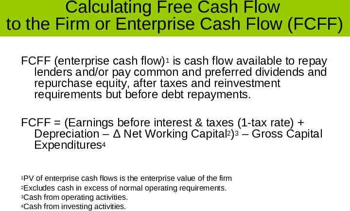
Calculating Free Cash Flow to the Firm or Enterprise Cash Flow (FCFF) FCFF (enterprise cash flow)1 is cash flow available to repay lenders and/or pay common and preferred dividends and repurchase equity, after taxes and reinvestment requirements but before debt repayments. FCFF (Earnings before interest & taxes (1-tax rate) Depreciation – Δ Net Working Capital2)3 – Gross Capital Expenditures4 PV of enterprise cash flows is the enterprise value of the firm 2Excludes cash in excess of normal operating requirements. 3Cash from operating activities. 4Cash from investing activities. 1
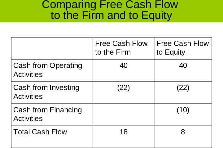
Comparing Free Cash Flow to the Firm and to Equity Free Cash Flow to the Firm Free Cash Flow to Equity Cash from Operating Activities 40 40 Cash from Investing Activities (22) (22) Cash from Financing Activities Total Cash Flow (10) 18 8
Discussion Questions 1. How does the size of the firm affect its perceived risk? Be specific? 2. How would you estimate the beta for a publicly traded firm? For a private firm? 3. Explain the difference between equity and enterprise cash flow? 4. What is the appropriate discount rate to use with equity cash flow? Why? With enterprise cash flow? Why?
Commonly Used Discounted Cash Flow Valuation Methods Zero Growth Model Constant Growth Model Variable Growth Model
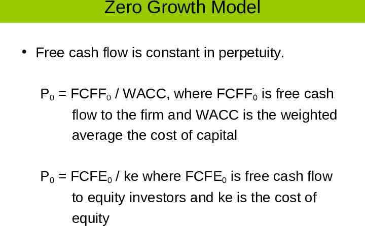
Zero Growth Model Free cash flow is constant in perpetuity. P0 FCFF0 / WACC, where FCFF0 is free cash flow to the firm and WACC is the weighted average the cost of capital P0 FCFE0 / ke where FCFE0 is free cash flow to equity investors and ke is the cost of equity
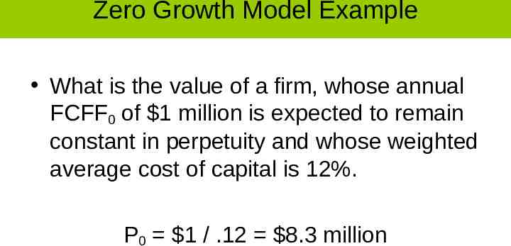
Zero Growth Model Example What is the value of a firm, whose annual FCFF0 of 1 million is expected to remain constant in perpetuity and whose weighted average cost of capital is 12%. P0 1 / .12 8.3 million
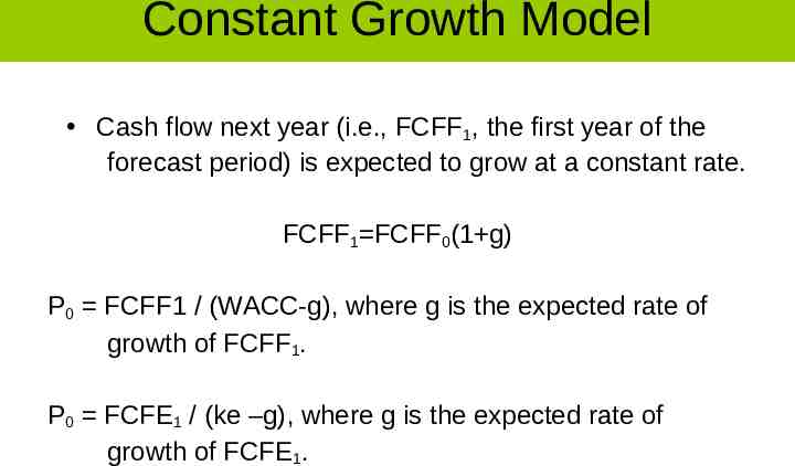
Constant Growth Model Cash flow next year (i.e., FCFF1, the first year of the forecast period) is expected to grow at a constant rate. FCFF1 FCFF0(1 g) P0 FCFF1 / (WACC-g), where g is the expected rate of growth of FCFF1. P0 FCFE1 / (ke –g), where g is the expected rate of growth of FCFE1.
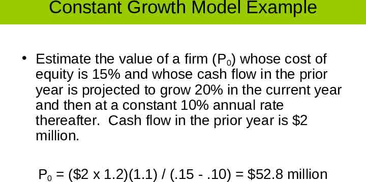
Constant Growth Model Example Estimate the value of a firm (P0) whose cost of equity is 15% and whose cash flow in the prior year is projected to grow 20% in the current year and then at a constant 10% annual rate thereafter. Cash flow in the prior year is 2 million. P0 ( 2 x 1.2)(1.1) / (.15 - .10) 52.8 million
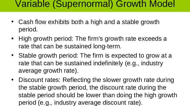
Variable (Supernormal) Growth Model Cash flow exhibits both a high and a stable growth period. High growth period: The firm’s growth rate exceeds a rate that can be sustained long-term. Stable growth period: The firm is expected to grow at a rate that can be sustained indefinitely (e.g., industry average growth rate). Discount rates: Reflecting the slower growth rate during the stable growth period, the discount rate during the stable period should be lower than doing the high growth period (e.g., industry average discount rate).
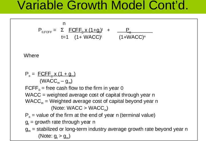
Variable Growth Model Cont’d. n P0,FCFF Σ FCFF0 x (1 gt)t t 1 (1 WACC)t Pn (1 WACC)n Where Pn FCFFn x (1 gm) (WACCm – gm) FCFF0 free cash flow to the firm in year 0 WACC weighted average cost of capital through year n WACCm Weighted average cost of capital beyond year n (Note: WACC WACCm) Pn value of the firm at the end of year n (terminal value) gt growth rate through year n gm stabilized or long-term industry average growth rate beyond year n (Note: gt gm)
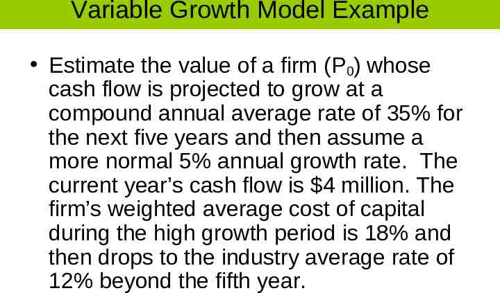
Variable Growth Model Example Estimate the value of a firm (P0) whose cash flow is projected to grow at a compound annual average rate of 35% for the next five years and then assume a more normal 5% annual growth rate. The current year’s cash flow is 4 million. The firm’s weighted average cost of capital during the high growth period is 18% and then drops to the industry average rate of 12% beyond the fifth year.
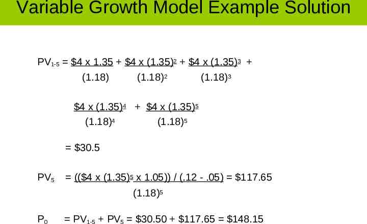
Variable Growth Model Example Solution PV1-5 4 x 1.35 4 x (1.35)2 4 x (1.35)3 (1.18) (1.18)2 (1.18)3 4 x (1.35)4 4 x (1.35)5 (1.18)4 (1.18)5 30.5 PV5 (( 4 x (1.35)5 x 1.05)) / (.12 - .05) 117.65 (1.18)5 P0 PV1-5 PV5 30.50 117.65 148.15
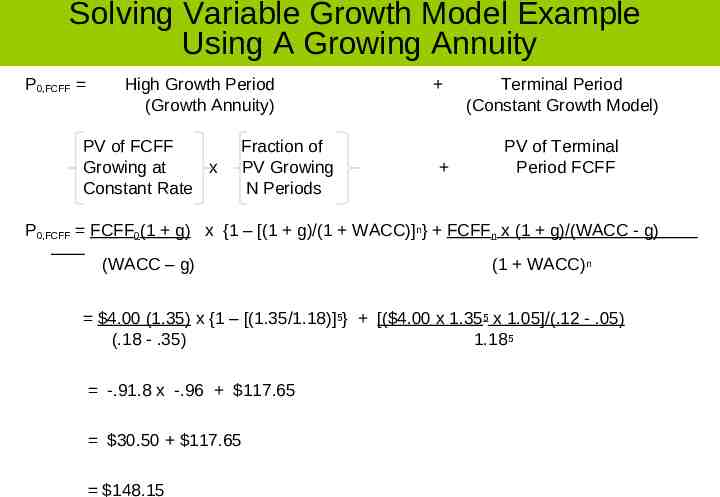
Solving Variable Growth Model Example Using A Growing Annuity P0,FCFF High Growth Period (Growth Annuity) PV of FCFF Growing at x Constant Rate Fraction of PV Growing N Periods Terminal Period (Constant Growth Model) PV of Terminal Period FCFF P0,FCFF FCFF0(1 g) x {1 – [(1 g)/(1 WACC)]n} FCFFn x (1 g)/(WACC - g) (WACC – g) (1 WACC) n 4.00 (1.35) x {1 – [(1.35/1.18)]5} [( 4.00 x 1.355 x 1.05]/(.12 - .05) (.18 - .35) 1.18 5 -.91.8 x -.96 117.65 30.50 117.65 148.15
Determining Growth Rates Key premise: A firm’s value can be approximated by the sum of the high growth plus a stable growth period. Key risks: Sensitivity of terminal values to choice of assumptions about stable growth rate and discount rates used in both the terminal and annual cash flow periods. Stable growth rate: The firm’s growth rate that is expected to last forever. Generally equal to or less than the industry or overall economy’s growth rate. For multinational firms, the growth rate is the world economy’s rate of growth. Length of the high growth period: The greater the current growth rate of a firm’s cash flow relative to the stable growth rate, the longer the high growth period.
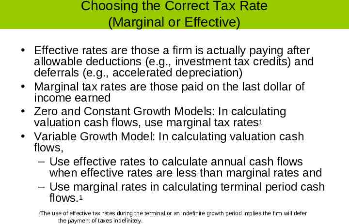
Choosing the Correct Tax Rate (Marginal or Effective) Effective rates are those a firm is actually paying after allowable deductions (e.g., investment tax credits) and deferrals (e.g., accelerated depreciation) Marginal tax rates are those paid on the last dollar of income earned Zero and Constant Growth Models: In calculating valuation cash flows, use marginal tax rates1 Variable Growth Model: In calculating valuation cash flows, – Use effective rates to calculate annual cash flows when effective rates are less than marginal rates and – Use marginal rates in calculating terminal period cash flows.1 The use of effective tax rates during the terminal or an indefinite growth period implies the firm will defer the payment of taxes indefinitely. 1
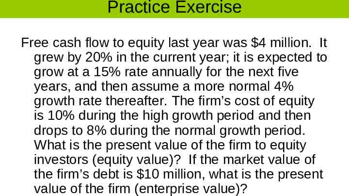
Practice Exercise Free cash flow to equity last year was 4 million. It grew by 20% in the current year; it is expected to grow at a 15% rate annually for the next five years, and then assume a more normal 4% growth rate thereafter. The firm’s cost of equity is 10% during the high growth period and then drops to 8% during the normal growth period. What is the present value of the firm to equity investors (equity value)? If the market value of the firm’s debt is 10 million, what is the present value of the firm (enterprise value)?
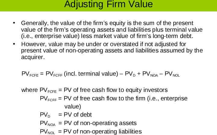
Adjusting Firm Value Generally, the value of the firm’s equity is the sum of the present value of the firm’s operating assets and liabilities plus terminal value (i.e., enterprise value) less market value of firm’s long-term debt. However, value may be under or overstated if not adjusted for present value of non-operating assets and liabilities assumed by the acquirer. PVFCFE PVFCFF (incl. terminal value) – PVD PVNOA – PVNOL where PVFCFE PV of free cash flow to equity investors PVFCFF PV of free cash flow to the firm (i.e., enterprise value) PVD PV of debt PVNOA PV of non-operating assets PVNOL PV of non-operating liabilities
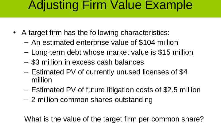
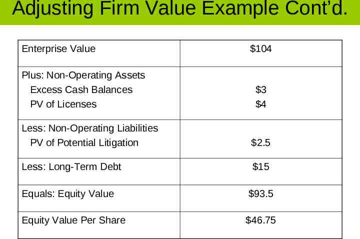
Adjusting Firm Value Example A target firm has the following characteristics: – An estimated enterprise value of 104 million – Long-term debt whose market value is 15 million – 3 million in excess cash balances – Estimated PV of currently unused licenses of 4 million – Estimated PV of future litigation costs of 2.5 million – 2 million common shares outstanding What is the value of the target firm per common share?
Adjusting Firm Value Example Cont’d. Enterprise Value Plus: Non-Operating Assets Excess Cash Balances PV of Licenses 104 3 4 Less: Non-Operating Liabilities PV of Potential Litigation 2.5 Less: Long-Term Debt 15 Equals: Equity Value 93.5 Equity Value Per Share 46.75
Things to Remember Zero growth model: Cash flow is expected to remain constant in perpetuity. Constant growth model: Cash flow is expected to grow at a constant rate. Variable (supernormal) growth model: Cash flow exhibits both a high and a stable growth period. – Total present value represents the sum of the discounted value of the cash flows over both periods. – The terminal value frequently accounts for most of the total present value calculation and is highly sensitive to the choice of growth and discount rates.