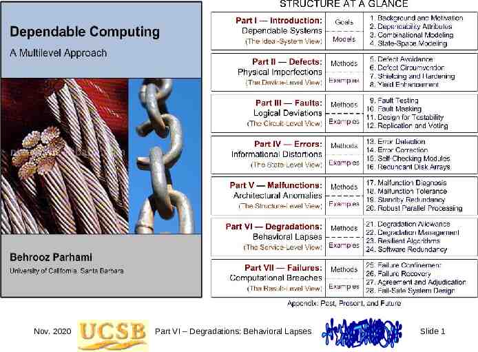
Nov. 2020 Part VI – Degradations: Behavioral Lapses Slide 1


78 Slides3.10 MB
Nov. 2020 Part VI – Degradations: Behavioral Lapses Slide 1
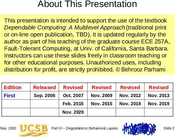
About This Presentation This presentation is intended to support the use of the textbook Dependable Computing: A Multilevel Approach (traditional print or on-line open publication, TBD). It is updated regularly by the author as part of his teaching of the graduate course ECE 257A, Fault-Tolerant Computing, at Univ. of California, Santa Barbara. Instructors can use these slides freely in classroom teaching or for other educational purposes. Unauthorized uses, including distribution for profit, are strictly prohibited. Behrooz Parhami Edition Released Revised Revised Revised Revised First Sep. 2006 Oct. 2007 Nov. 2009 Nov. 2012 Nov. 2013 Feb. 2015 Nov. 2015 Nov. 2018 Nov. 2019 Nov. 2020 Nov. 2020 Part VI – Degradations: Behavioral Lapses Slide 2
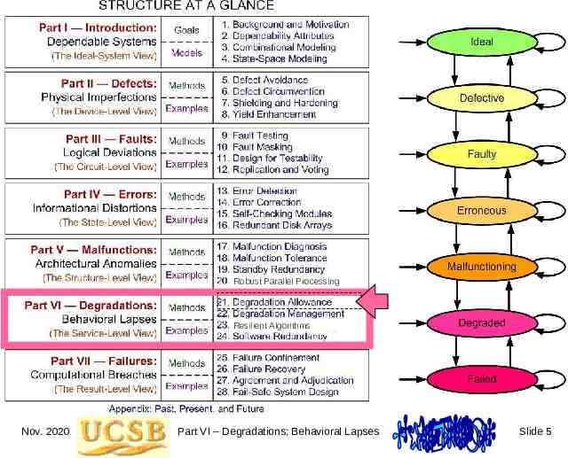
21 Degradation Allowance Nov. 2020 Part VI – Degradations: Behavioral Lapses Slide 3
“Redundancy is such an ugly word. Let’s talk about your ‘employment crunch’.” Our computers are down, so we have to do everything manually. Nov. 2020 Part VI – Degradations: Behavioral Lapses Slide 4
Robust Parallel Processing Resilient Algorithms Nov. 2020 Part VI – Degradations: Behavioral Lapses Slide 5
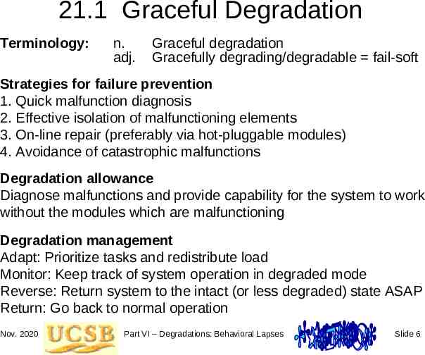
21.1 Graceful Degradation Terminology: n. adj. Graceful degradation Gracefully degrading/degradable fail-soft Strategies for failure prevention 1. Quick malfunction diagnosis 2. Effective isolation of malfunctioning elements 3. On-line repair (preferably via hot-pluggable modules) 4. Avoidance of catastrophic malfunctions Degradation allowance Diagnose malfunctions and provide capability for the system to work without the modules which are malfunctioning Degradation management Adapt: Prioritize tasks and redistribute load Monitor: Keep track of system operation in degraded mode Reverse: Return system to the intact (or less degraded) state ASAP Return: Go back to normal operation Nov. 2020 Part VI – Degradations: Behavioral Lapses Slide 6
Degradation Allowance Is Not Automatic A car possessing extra wheels compared with the minimum number required does not guarantee that it can operate with fewer wheels Nov. 2020 Part VI – Degradations: Behavioral Lapses Slide 7
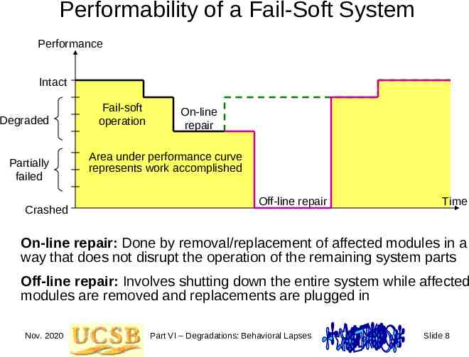
Performability of a Fail-Soft System Performance Intact Degraded Partially failed Crashed Fail-soft operation On-line repair Area under performance curve represents work accomplished Off-line repair Time On-line repair: Done by removal/replacement of affected modules in a way that does not disrupt the operation of the remaining system parts Off-line repair: Involves shutting down the entire system while affected modules are removed and replacements are plugged in Nov. 2020 Part VI – Degradations: Behavioral Lapses Slide 8
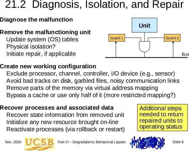
21.2 Diagnosis, Isolation, and Repair Diagnose the malfunction Remove the malfunctioning unit Update system (OS) tables Physical isolation? Initiate repair, if applicable Unit Guard 1 Guard 2 Bus Create new working configuration Exclude processor, channel, controller, I/O device (e.g., sensor) Avoid bad tracks on disk, garbled files, noisy communication links Remove parts of the memory via virtual address mapping Bypass a cache or use only half of it (more restricted mapping?) Recover processes and associated data Recover state information from removed unit Initialize any new resource brought on-line Reactivate processes (via rollback or restart) Nov. 2020 Part VI – Degradations: Behavioral Lapses Additional steps needed to return repaired units to operating status Slide 9
21.3 Stable Storage Storage that won’t lose its contents (unlike registers and SRAM/DRAM) Possible implementation method: Battery backup for a time duration long enough to save contents of disk cache or other volatile memory Flash memory Combined stability & reliability can be provided with RAID-like methods Nov. 2020 Part VI – Degradations: Behavioral Lapses Slide 10
Malfunction-Stop Modules Malfunction tolerance would be much easier if modules simply stopped functioning, rather than engage in arbitrary behavior Unpredictable (Byzantine) malfunctions are notoriously hard to handle Assuming the availability of a reliable stable storage along with its controlling s-process and (approximately) synchronized clocks, a k-malfunction-stop module can be implemented from k 1 units Operation of s-process to decide whether the module has stopped: R : bag of received requests with appropriate timestamps if R k 1 all requests identical and from different sources stop then if request is a write then perform the write operation in stable storage else if request is a read, send value to all processes else set variable stop in stable storage to TRUE Nov. 2020 Part VI – Degradations: Behavioral Lapses Slide 11
21.4 Process and Data Recovery Use of logs with process restart Impossible when the system operates in real time and performs actions that cannot be undone Such actions must be compensated for as part of degradation management Nov. 2020 Part VI – Degradations: Behavioral Lapses Slide 12
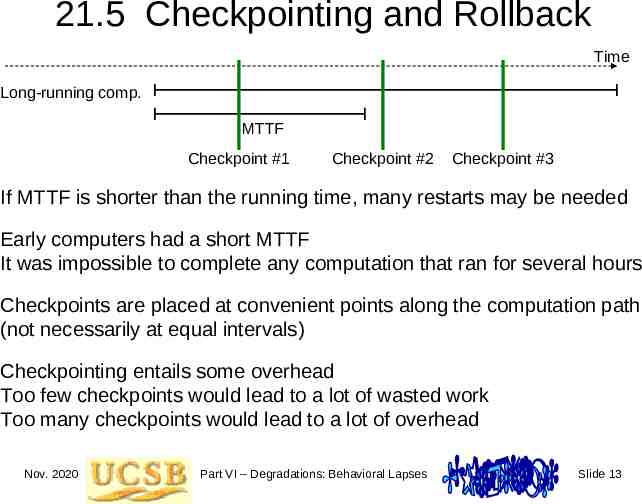
21.5 Checkpointing and Rollback Time Long-running comp. MTTF Checkpoint #1 Checkpoint #2 Checkpoint #3 If MTTF is shorter than the running time, many restarts may be needed Early computers had a short MTTF It was impossible to complete any computation that ran for several hours Checkpoints are placed at convenient points along the computation path (not necessarily at equal intervals) Checkpointing entails some overhead Too few checkpoints would lead to a lot of wasted work Too many checkpoints would lead to a lot of overhead Nov. 2020 Part VI – Degradations: Behavioral Lapses Slide 13
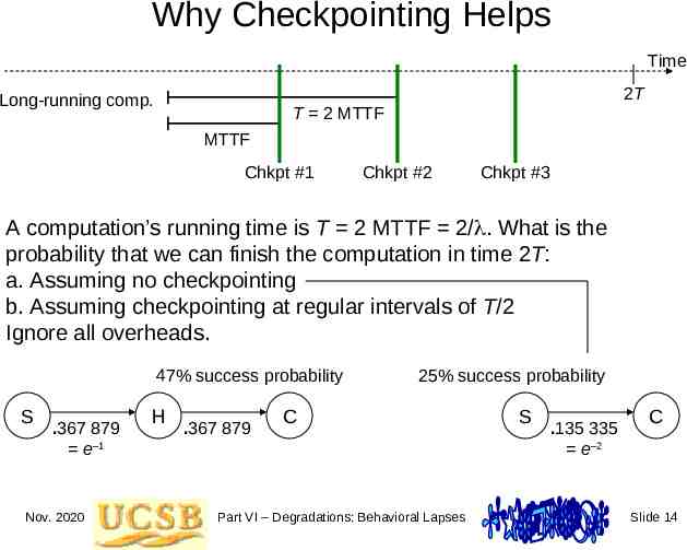
Why Checkpointing Helps Time 2T Long-running comp. T 2 MTTF MTTF Chkpt #1 Chkpt #2 Chkpt #3 A computation’s running time is T 2 MTTF 2/ . What is the probability that we can finish the computation in time 2T: a. Assuming no checkpointing b. Assuming checkpointing at regular intervals of T/2 Ignore all overheads. 47% success probability S .367 879 e–1 Nov. 2020 H .367 879 25% success probability C Part VI – Degradations: Behavioral Lapses S .135 335 e–2 C Slide 14
Recovery via Rollback Time Process 1 Process 2 Process 3 Process 4 Affected processes Process 5 Process 6 Checkpoint #1 Checkpoint #2 Detected malfunction Roll back process 2 to the last checkpoint (#2) Restart process 6 Rollback or restart creates no problem for tasks that do I/O at the end Interactive processes must be handled with more care e.g., bank ATM transaction to withdraw money or transfer funds (check balance, reduce balance, dispense cash or increase balance) Nov. 2020 Part VI – Degradations: Behavioral Lapses Slide 15
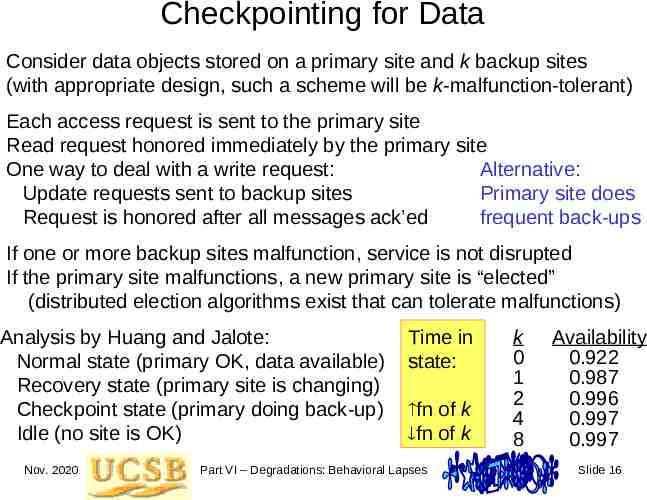
Checkpointing for Data Consider data objects stored on a primary site and k backup sites (with appropriate design, such a scheme will be k-malfunction-tolerant) Each access request is sent to the primary site Read request honored immediately by the primary site One way to deal with a write request: Alternative: Update requests sent to backup sites Primary site does Request is honored after all messages ack’ed frequent back-ups If one or more backup sites malfunction, service is not disrupted If the primary site malfunctions, a new primary site is “elected” (distributed election algorithms exist that can tolerate malfunctions) Analysis by Huang and Jalote: Normal state (primary OK, data available) Recovery state (primary site is changing) Checkpoint state (primary doing back-up) Idle (no site is OK) Nov. 2020 Time in state: fn of k fn of k Part VI – Degradations: Behavioral Lapses k 0 1 2 4 8 Availability 0.922 0.987 0.996 0.997 0.997 Slide 16
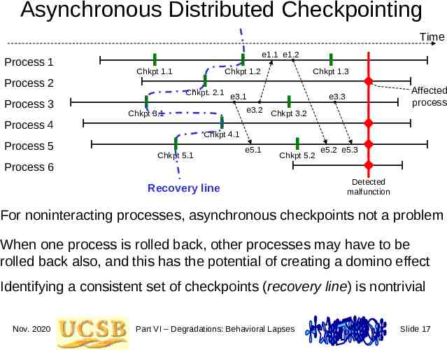
Asynchronous Distributed Checkpointing Time Process 1 I Chkpt 1.1 Process 2 Process 3 Chkpt 1.2 I Chkpt. 2.1 e3.1 I Chkpt 3.1 I Process 4 Process 5 e1.1 e1.2 I I Affected process e3.3 I e3.2 Chkpt 3.2 Chkpt 4.1 Chkpt 5.1 I Chkpt 1.3 e5.1 I Chkpt 5.2 e5.2 e5.3 Process 6 Recovery line Detected malfunction For noninteracting processes, asynchronous checkpoints not a problem When one process is rolled back, other processes may have to be rolled back also, and this has the potential of creating a domino effect Identifying a consistent set of checkpoints (recovery line) is nontrivial Nov. 2020 Part VI – Degradations: Behavioral Lapses Slide 17
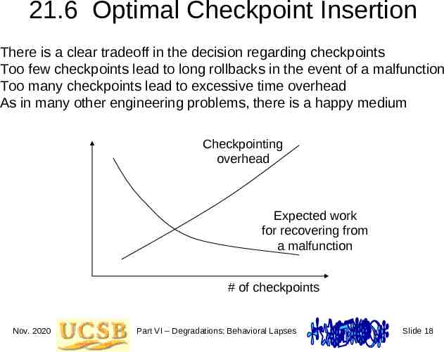
21.6 Optimal Checkpoint Insertion There is a clear tradeoff in the decision regarding checkpoints Too few checkpoints lead to long rollbacks in the event of a malfunction Too many checkpoints lead to excessive time overhead As in many other engineering problems, there is a happy medium Checkpointing overhead Expected work for recovering from a malfunction # of checkpoints Nov. 2020 Part VI – Degradations: Behavioral Lapses Slide 18
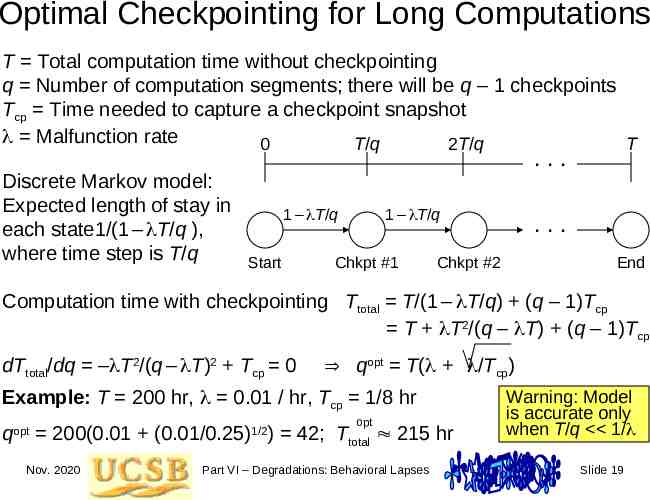
Optimal Checkpointing for Long Computations T Total computation time without checkpointing q Number of computation segments; there will be q – 1 checkpoints Tcp Time needed to capture a checkpoint snapshot Malfunction rate 0 T/q 2T/q T . . . Discrete Markov model: Expected length of stay in each state1/(1 – T/q ), where time step is T/q 1 – T/q Start 1 – T/q Chkpt #1 . . . Chkpt #2 End Computation time with checkpointing Ttotal T/(1 – T/q) (q – 1)Tcp T T2/(q – T) (q – 1)Tcp dTtotal/dq – T2/(q – T)2 Tcp 0 qopt T( /Tcp) Example: T 200 hr, 0.01 / hr, Tcp 1/8 hr q opt opt 200(0.01 (0.01/0.25) ) 42; Ttotal 215 hr Nov. 2020 1/2 Part VI – Degradations: Behavioral Lapses Warning: Model is accurate only when T/q 1/ Slide 19
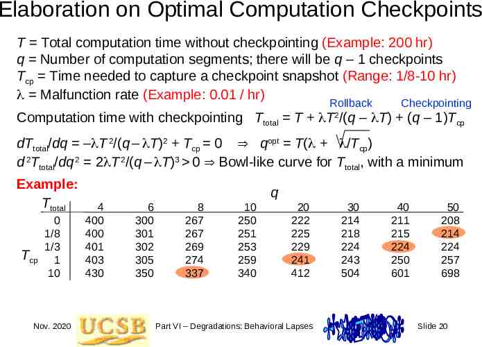
Elaboration on Optimal Computation Checkpoints T Total computation time without checkpointing (Example: 200 hr) q Number of computation segments; there will be q – 1 checkpoints Tcp Time needed to capture a checkpoint snapshot (Range: 1/8-10 hr) Malfunction rate (Example: 0.01 / hr) Rollback Checkpointing Computation time with checkpointing Ttotal T T2/(q – T) (q – 1)Tcp dTtotal/dq – T 2/(q – T)2 Tcp 0 qopt T( /Tcp) d 2Ttotal/dq 2 2 T 2/(q – T)3 0 Bowl-like curve for Ttotal, with a minimum Example: Ttotal 0 1/8 1/3 Tcp 1 10 100 1000 Nov. 2020 q 4 400 400 401 403 430 700 3400 6 300 301 302 305 350 800 5300 8 267 267 269 274 337 967 7267 10 250 251 253 259 340 1150 9250 20 222 225 229 241 412 2122 19222 Part VI – Degradations: Behavioral Lapses 30 214 218 224 243 504 3114 29214 40 211 215 224 250 601 4111 39211 50 208 214 224 257 698 5108 49208 Slide 20
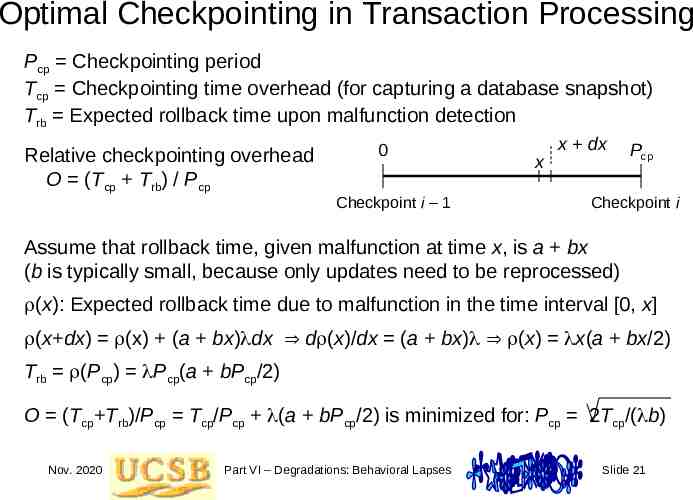
Optimal Checkpointing in Transaction Processing Pcp Checkpointing period Tcp Checkpointing time overhead (for capturing a database snapshot) Trb Expected rollback time upon malfunction detection Relative checkpointing overhead O (Tcp Trb) / Pcp 0 Checkpoint i – 1 x x dx Pcp Checkpoint i Assume that rollback time, given malfunction at time x, is a bx (b is typically small, because only updates need to be reprocessed) (x): Expected rollback time due to malfunction in the time interval [0, x] (x dx) (x) (a bx) dx d (x)/dx (a bx) (x) x(a bx/2) Trb (Pcp) Pcp(a bPcp/2) O (Tcp Trb)/Pcp Tcp/Pcp (a bPcp/2) is minimized for: Pcp 2Tcp/( b) Nov. 2020 Part VI – Degradations: Behavioral Lapses Slide 21
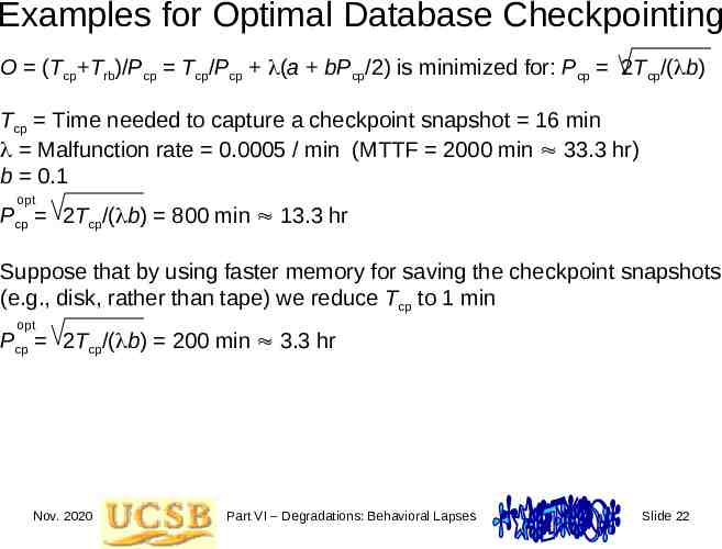
Examples for Optimal Database Checkpointing O (Tcp Trb)/Pcp Tcp/Pcp (a bPcp/2) is minimized for: Pcp 2Tcp/( b) Tcp Time needed to capture a checkpoint snapshot 16 min Malfunction rate 0.0005 / min (MTTF 2000 min 33.3 hr) b 0.1 opt Pcp 2Tcp/( b) 800 min 13.3 hr Suppose that by using faster memory for saving the checkpoint snapshots (e.g., disk, rather than tape) we reduce Tcp to 1 min opt Pcp 2Tcp/( b) 200 min 3.3 hr Nov. 2020 Part VI – Degradations: Behavioral Lapses Slide 22
22 Degradation Management Nov. 2020 Part VI – Degradations: Behavioral Lapses Slide 23
“Budget cuts.” Nov. 2020 Part VI – Degradations: Behavioral Lapses Slide 24
Robust Parallel Processing Resilient Algorithms Nov. 2020 Part VI – Degradations: Behavioral Lapses Slide 25
22.1 Data Distribution Methods Reliable data storage requires that the availability and integrity of data not be dependent on the health of any one site Data Replication Data dispersion Nov. 2020 Part VI – Degradations: Behavioral Lapses Slide 26
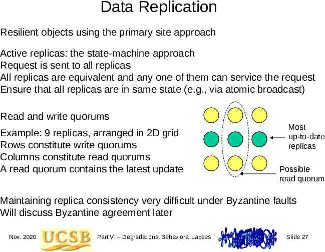
Data Replication Resilient objects using the primary site approach Active replicas: the state-machine approach Request is sent to all replicas All replicas are equivalent and any one of them can service the request Ensure that all replicas are in same state (e.g., via atomic broadcast) Read and write quorums Example: 9 replicas, arranged in 2D grid Rows constitute write quorums Columns constitute read quorums A read quorum contains the latest update Most up-to-date replicas Possible read quorum Maintaining replica consistency very difficult under Byzantine faults Will discuss Byzantine agreement later Nov. 2020 Part VI – Degradations: Behavioral Lapses Slide 27
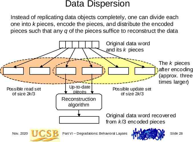
Data Dispersion Instead of replicating data objects completely, one can divide each one into k pieces, encode the pieces, and distribute the encoded pieces such that any q of the pieces suffice to reconstruct the data Original data word and its k pieces Possible read set of size 2k/3 Up-to-date pieces Reconstruction Recunstruction algorithm algorithm The k pieces after encoding (approx. three times larger) Possible update set of size 2k/3 Original data word recovered from k /3 encoded pieces Nov. 2020 Part VI – Degradations: Behavioral Lapses Slide 28
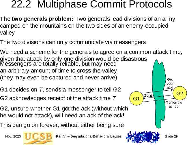
22.2 Multiphase Commit Protocols The two generals problem: Two generals lead divisions of an army camped on the mountains on the two sides of an enemy-occupied valley The two divisions can only communicate via messengers We need a scheme for the generals to agree on a common attack time, given that attack by only one division would be disastrous Messengers are totally reliable, but may need an arbitrary amount of time to cross the valley (they may even be captured and never arrive) Got G1 decides on T, sends a messenger to tell G2 G2 acknowledges receipt of the attack time T G2, unsure whether G1 got the ack (without which he would not attack), will need an ack of the ack! your ack! G1 Got it! G2 Tomorrow at noon This can go on forever, without either being sure Nov. 2020 Part VI – Degradations: Behavioral Lapses Slide 29
Maintaining System Consistency Atomic action: Either the entire action is completed or none of it is done One key tool is the ability to ensure atomicity despite malfunctions Similar to a computer guaranteeing sequential execution of instructions, even though it may perform some steps in parallel or out of order Where atomicity is useful: Upon a write operation, ensure that all data replicas are updated Electronic funds transfer (reduce one balance, increase the other one) In centralized systems atomicity can be ensured via locking mechanisms Acquire (read or write) lock for desired data object and operation Perform operation Release lock A key challenge of locks is to avoid deadlock (circular waiting for locks) Nov. 2020 Part VI – Degradations: Behavioral Lapses Slide 30
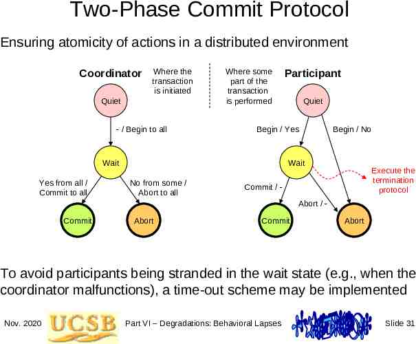
Two-Phase Commit Protocol Ensuring atomicity of actions in a distributed environment Coordinator Where the transaction is initiated Quiet / Begin to all Where some part of the transaction is performed Quiet Begin / Yes Wait Yes from all / Commit to all Participant Begin / No Wait No from some / Abort to all Execute the termination protocol Commit / Abort / Commit Abort Commit Abort To avoid participants being stranded in the wait state (e.g., when the coordinator malfunctions), a time-out scheme may be implemented Nov. 2020 Part VI – Degradations: Behavioral Lapses Slide 31
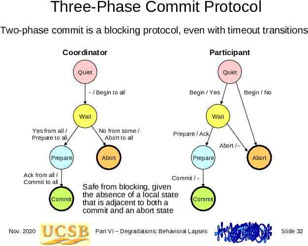
Three-Phase Commit Protocol Two-phase commit is a blocking protocol, even with timeout transitions Coordinator Participant Quiet Quiet / Begin to all Begin / Yes Wait Yes from all / Prepare to all Begin / No Wait No from some / Abort to all Prepare / Ack Abort / Prepare Ack from all / Commit to all Commit Nov. 2020 Abort Prepare Abort Commit / Safe from blocking, given the absence of a local state that is adjacent to both a commit and an abort state Commit Part VI – Degradations: Behavioral Lapses Slide 32
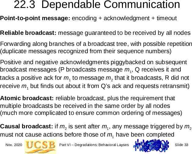
22.3 Dependable Communication Point-to-point message: encoding acknowledgment timeout Reliable broadcast: message guaranteed to be received by all nodes Forwarding along branches of a broadcast tree, with possible repetition (duplicate messages recognized from their sequence numbers) Positive and negative acknowledgments piggybacked on subsequent broadcast messages (P broadcasts message m1, Q receives it and tacks a positive ack for m1 to message m2 that it broadcasts, R did not receive m1 but finds out about it from Q’s ack and requests retransmit) Atomic broadcast: reliable broadcast, plus the requirement that multiple broadcasts be received in the same order by all nodes (much more complicated to ensure common ordering of messages) Causal broadcast: if m2 is sent after m1, any message triggered by m2 must not cause actions before those of m1 have been completed Nov. 2020 Part VI – Degradations: Behavioral Lapses Slide 33
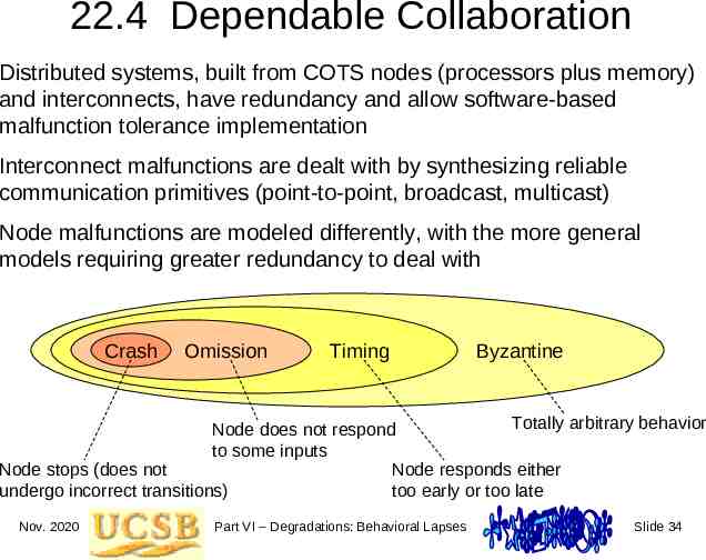
22.4 Dependable Collaboration Distributed systems, built from COTS nodes (processors plus memory) and interconnects, have redundancy and allow software-based malfunction tolerance implementation Interconnect malfunctions are dealt with by synthesizing reliable communication primitives (point-to-point, broadcast, multicast) Node malfunctions are modeled differently, with the more general models requiring greater redundancy to deal with Crash Omission Timing Byzantine Totally arbitrary behavior Node does not respond to some inputs Node stops (does not Node responds either undergo incorrect transitions) too early or too late Nov. 2020 Part VI – Degradations: Behavioral Lapses Slide 34
Malfunction Detectors in Distributed Systems Malfunction detector: Distributed oracle related to malfunction detection Creates and maintains a list of suspected processes Defined by two properties: completeness and accuracy Advantages: Allows decoupling of the effort to detect malfunctions, e.g. site crashes, from that of the actual computation, leading to more modular design Improves portability, because the same application can be used on a different platform if suitable malfunction detectors are available for it Example malfunction detectors: P (Perfect): strong completeness, strong accuracy (min required for IC) S: strong completeness, eventual weak accuracy (min for consensus) Reference: M. Raynal, “A Short Introduction to Failure Detectors for Asynchronous Distributed Systems,” ACM SIGACT News, Vol. 36, No. 1, pp. 53-70, March 2005. Nov. 2020 Part VI – Degradations: Behavioral Lapses Slide 35
Reliable Group Membership Service A group of processes may be cooperating for solving a problem The group’s membership may expand and contract owing to changing processing requirements or because of malfunctions and repairs Reliable multicast: message guaranteed to be received by all members within the group ECE 254C: Advanced Computer Architecture – Distributed Systems (course devoted to distributed computing and its reliability issues) Nov. 2020 Part VI – Degradations: Behavioral Lapses Slide 36
22.5 Remapping and Load Balancing When pieces of a computation are performed on different modules, remapping may expose hidden malfunctions After remapping, various parts of the computation are performed by different modules compared with the original mapping It is quite unlikely that the same incorrect answers are obtained in the remapped version Load balancing is the act of redistributing the computational load in the face of lost/recovered resources and dynamically changing computational requirements Nov. 2020 Part VI – Degradations: Behavioral Lapses Slide 37
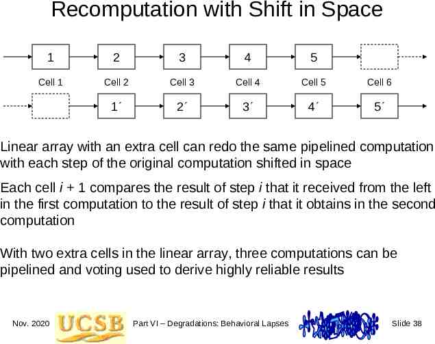
Recomputation with Shift in Space 1 2 3 4 5 Cell 1 Cell 2 Cell 3 Cell 4 Cell 5 Cell 6 1 2 3 4 5 Linear array with an extra cell can redo the same pipelined computation with each step of the original computation shifted in space Each cell i 1 compares the result of step i that it received from the left in the first computation to the result of step i that it obtains in the second computation With two extra cells in the linear array, three computations can be pipelined and voting used to derive highly reliable results Nov. 2020 Part VI – Degradations: Behavioral Lapses Slide 38
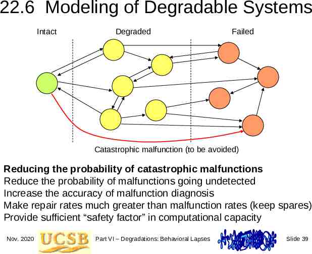
22.6 Modeling of Degradable Systems Intact Degraded Failed Catastrophic malfunction (to be avoided) Reducing the probability of catastrophic malfunctions Reduce the probability of malfunctions going undetected Increase the accuracy of malfunction diagnosis Make repair rates much greater than malfunction rates (keep spares) Provide sufficient “safety factor” in computational capacity Nov. 2020 Part VI – Degradations: Behavioral Lapses Slide 39
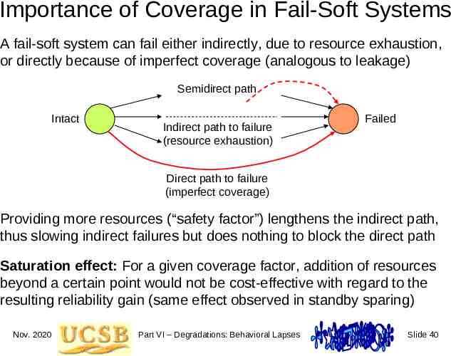
Importance of Coverage in Fail-Soft Systems A fail-soft system can fail either indirectly, due to resource exhaustion, or directly because of imperfect coverage (analogous to leakage) Semidirect path Intact Indirect path to failure (resource exhaustion) Failed Direct path to failure (imperfect coverage) Providing more resources (“safety factor”) lengthens the indirect path, thus slowing indirect failures but does nothing to block the direct path Saturation effect: For a given coverage factor, addition of resources beyond a certain point would not be cost-effective with regard to the resulting reliability gain (same effect observed in standby sparing) Nov. 2020 Part VI – Degradations: Behavioral Lapses Slide 40
23 Resilient Algorithms Nov. 2020 Part VI – Degradations: Behavioral Lapses Slide 41
“Just a darn minute! Yesterday you said X equals two!” Nov. 2020 Part VI – Degradations: Behavioral Lapses Slide 42
Robust Parallel Processing Resilient Algorithms Nov. 2020 Part VI – Degradations: Behavioral Lapses Slide 43
23.1 COTS-Based Paradigms Many of the hardware and software redundancy methods assume that we are building the entire system (or a significant part of it) from scratch Some companies with fault-tolerant systems and related services: ARM: Fault-tolerant ARM (launched in late 2006), automotive applications Nth Generation Computing: High-availability and enterprise storage systems Resilience Corp.: Emphasis on data security Stratus Technologies: “The Availability Company” Sun Microsystems: Fault-tolerant SPARC ( ft-SPARC ) Tandem Computers: An early ft leader, part of HP/Compaq since 1997 Question: What can be done to ensure the dependability of computations using commercial off-the-shelf (COTS) components? A number of algorithm and data-structure design methods are available Nov. 2020 Part VI – Degradations: Behavioral Lapses Slide 44
Some History: The SIFT Experience SIFT (software-implemented fault tolerance), developed at Stanford in early 1970s using mostly COTS components, was one of two competing “concept systems” for fly-by-wire aircraft control The other one, FTMP (fault-tolerant multiprocessor), developed at MIT, used a hardware-intensive approach System failure rate goal: 10–9/hr over a 10-hour flight SIFT allocated tasks for execution on multiple, loosely synchronized COTS processor-memory pairs (skew of up to 50 s was acceptable); only the bus system was custom designed Some fundamental results on, and methods for, clock synchronization emerged from this project To prevent errors from propagating, processors obtained multiple copies of data from different memories over different buses (local voting) Nov. 2020 Part VI – Degradations: Behavioral Lapses Slide 45
Limitations of the COTS-Based Approach Some modern microprocessors have dependability features built in: Parity and other codes in memory, TLB, microcode store Retry at various levels, from bus transmissions to full instructions Machine check facilities and registers to hold the check results According to Avizienis [Aviz97], however: These are often not documented enough to allow users to build on them Protection is nonsystematic and uneven Recovery options are limited to shutdown and restart Description of error handling is scattered among a lot of other detail There is no top-down view of the features and their interrelationships Manufacturers can incorporate both more advanced and new features, and at times have experimented with a number of mechanisms, but the low volume of the application base has hindered commercial viability Nov. 2020 Part VI – Degradations: Behavioral Lapses Slide 46
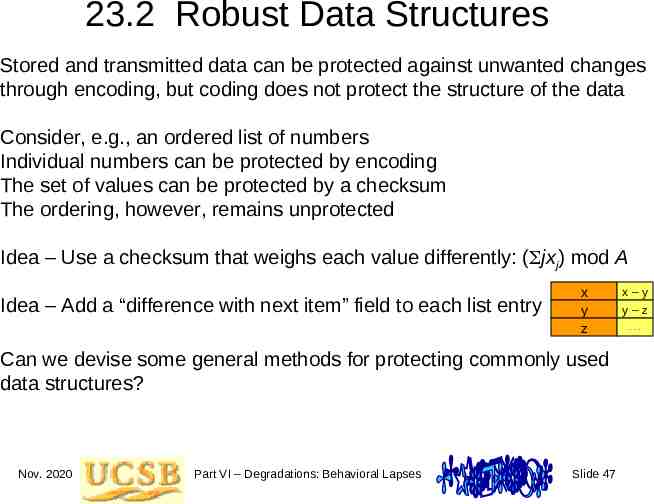
23.2 Robust Data Structures Stored and transmitted data can be protected against unwanted changes through encoding, but coding does not protect the structure of the data Consider, e.g., an ordered list of numbers Individual numbers can be protected by encoding The set of values can be protected by a checksum The ordering, however, remains unprotected Idea – Use a checksum that weighs each value differently: ( jxj) mod A Idea – Add a “difference with next item” field to each list entry x y z Can we devise some general methods for protecting commonly used data structures? Nov. 2020 Part VI – Degradations: Behavioral Lapses Slide 47 x–y y–z .
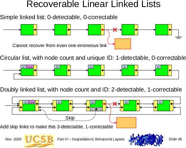
Recoverable Linear Linked Lists Simple linked list: 0-detectable, 0-correctable Cannot recover from even one erroneous link Circular list, with node count and unique ID: 1-detectable, 0-correctable ID Size ID ID ID ID Doubly linked list, with node count and ID: 2-detectable, 1-correctable ID Size ID ID ID ID Skip Add skip links to make this 3-detectable, 1-correctable Nov. 2020 Part VI – Degradations: Behavioral Lapses Slide 48
Other Robust Data Structures Trees, FIFOs, stacks (LIFOs), heaps, queues In general, a linked data structure is 2-detectable and 1-correctable iff the link network is 2-connected Robust data structures provide fairly good protection with little design effort or run-time overhead Audits can be performed during idle time Reuse possibility makes the method even more effective Robustness features to protect the structure can be combined with coding methods (such as checksums) to protect the content Nov. 2020 Part VI – Degradations: Behavioral Lapses Slide 49
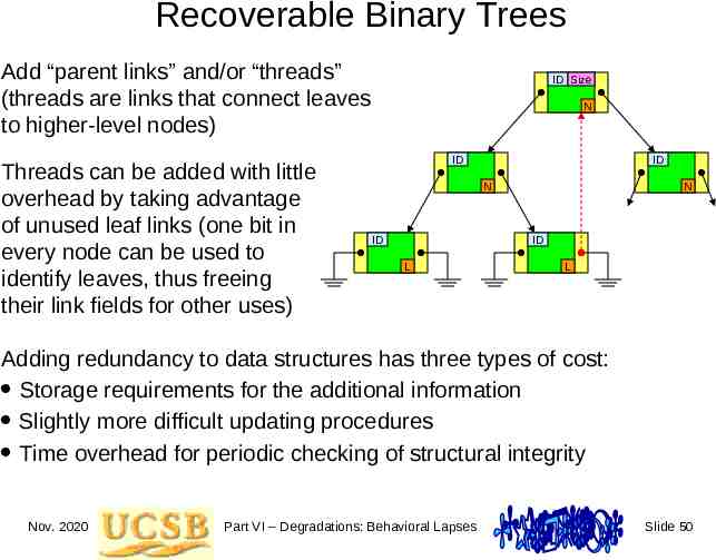
Recoverable Binary Trees Add “parent links” and/or “threads” (threads are links that connect leaves to higher-level nodes) Threads can be added with little overhead by taking advantage of unused leaf links (one bit in every node can be used to identify leaves, thus freeing their link fields for other uses) ID Size N ID ID N ID N ID L L Adding redundancy to data structures has three types of cost: Storage requirements for the additional information Slightly more difficult updating procedures Time overhead for periodic checking of structural integrity Nov. 2020 Part VI – Degradations: Behavioral Lapses Slide 50
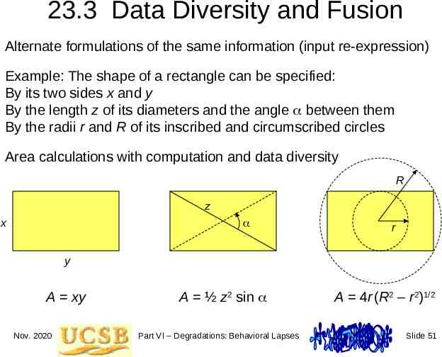
23.3 Data Diversity and Fusion Alternate formulations of the same information (input re-expression) Example: The shape of a rectangle can be specified: By its two sides x and y By the length z of its diameters and the angle between them By the radii r and R of its inscribed and circumscribed circles Area calculations with computation and data diversity R z x r y A xy Nov. 2020 A ½ z2 sin Part VI – Degradations: Behavioral Lapses A 4r (R2 – r2)1/2 Slide 51
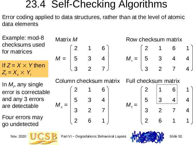
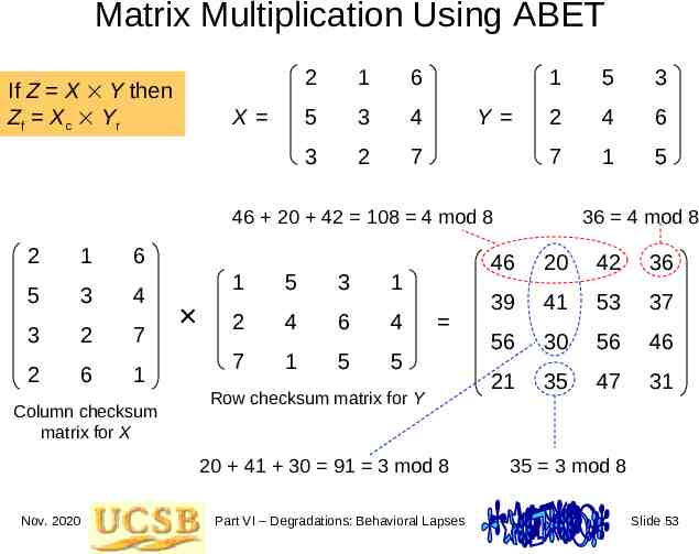
23.4 Self-Checking Algorithms Error coding applied to data structures, rather than at the level of atomic data elements Example: mod-8 checksums used for matrices If Z X Y then Zf Xc Yr Matrix M 2 1 6 Row checksum matrix 2 1 6 1 M 5 3 4 Mr 3 2 7 Column checksum matrix In Mf, any single 2 1 6 error is correctable and any 3 errors 5 3 4 Mc are detectable 3 2 7 Four errors may 2 6 1 go undetected Nov. 2020 5 3 4 4 3 2 7 4 Full checksum matrix 2 1 6 Mf Part VI – Degradations: Behavioral Lapses 1 5 3 4 4 3 2 7 4 2 6 1 1 Slide 52
Matrix Multiplication Using ABET If Z X Y then Zf Xc Yr X 2 1 6 5 3 4 3 2 7 Y 1 5 3 2 4 6 7 1 5 46 20 42 108 4 mod 8 2 1 6 5 3 4 3 2 7 2 6 1 Column checksum matrix for X 1 5 3 1 2 4 6 4 7 1 5 5 Row checksum matrix for Y 20 41 30 91 3 mod 8 Nov. 2020 Part VI – Degradations: Behavioral Lapses 36 4 mod 8 46 20 42 36 39 41 53 37 56 30 56 46 21 35 47 31 35 3 mod 8 Slide 53
23.5 Self-Adapting Algorithms This section to be completed Nov. 2020 Part VI – Degradations: Behavioral Lapses Slide 54
23.6 Other Algorithmic Methods This section to be completed Nov. 2020 Part VI – Degradations: Behavioral Lapses Slide 55
24 Software Redundancy Nov. 2020 Part VI – Degradations: Behavioral Lapses Slide 56
“Well, what’s a piece of software without a bug or two?” “We are neither hardware nor software; we are your parents.” “I haven’t the slightest idea who he is. He came bundled with the software.” Nov. 2020 Part VI – Degradations: Behavioral Lapses Slide 57
Robust Parallel Processing Resilient Algorithms Nov. 2020 Part VI – Degradations: Behavioral Lapses Slide 58
24.1 Software Dependability Imagine the following product disclaimers: For a steam iron There is no guarantee, explicit or implied, that this device will remove wrinkles from clothing or that it will not lead to the user’s electrocution. The manufacturer is not liable for any bodily harm or property damage resulting from the operation of this device. For an electric toaster The name “toaster” for this product is just a symbolic identifier. There is no guarantee, explicit or implied, that the device will prepare toast. Bread slices inserted in the product may be burnt from time to time, triggering smoke detectors or causing fires. By opening the package, the user acknowledges that s/he is willing to assume sole responsibility for any damages resulting from the product’s operation. Nov. 2020 Part VI – Degradations: Behavioral Lapses Slide 59
How Is Software Different from Hardware? Software unreliability is caused predominantly by design slips, not by operational deviations – we use flaw or bug, rather than fault or error Not much sense in replicating the same software and doing comparison or voting, as we did for hardware At the current levels of hardware complexity, latent design slips also exist in hardware, thus the two aren’t totally dissimilar The curse of complexity The 7-Eleven convenience store chain spent nearly 9M to make its point-of-sale software Y2K-compliant for its 5200 stores The modified software was subjected to 10,000 tests (all successful) The system worked with no problems throughout the year 2000 On January 1, 2001, however, the system began rejecting credit cards, because it “thought” the year was 1901 (bug was fixed within a day) Nov. 2020 Part VI – Degradations: Behavioral Lapses Slide 60
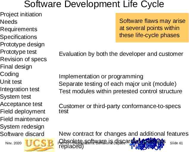
Software Development Life Cycle Project initiation Needs Requirements Specifications Prototype design Prototype test Revision of specs Final design Coding Unit test Integration test System test Acceptance test Field deployment Field maintenance System redesign Software discard Nov. 2020 Software flaws may arise at several points within these life-cycle phases Evaluation by both the developer and customer Implementation or programming Separate testing of each major unit (module) Test modules within pretested control structure Customer or third-party conformance-to-specs test New contract for changes and additional features Obsolete software is Lapses discarded (perhaps Slide 61 Part VI – Degradations: Behavioral replaced)
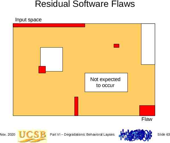
What Is Software Dependability? Major structural and logical problems are removed very early in the process of software testing What remains after extensive verification and validation is a collection of tiny flaws which surface under rare conditions or particular combinations of circumstances, thus giving software failure a statistical nature Software usually contains one or more flaws per thousand lines of code, with 1 flaw considered good (linux has been estimated to have 0.1) If there are f flaws in a software component, the hazard rate, that is, rate of failure occurrence per hour, is kf, with k being the constant of proportionality which is determined experimentally (e.g., k 0.0001) Software reliability: R(t) e–kft The only way to improve software reliability is to reduce the number of residual flaws through more rigorous verification and/or testing Nov. 2020 Part VI – Degradations: Behavioral Lapses Slide 62
Residual Software Flaws Input space Not expected to occur Flaw Nov. 2020 Part VI – Degradations: Behavioral Lapses Slide 63
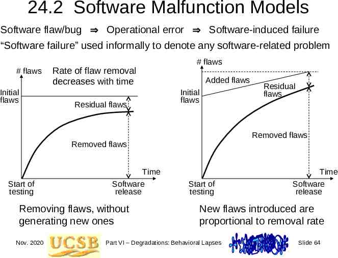
24.2 Software Malfunction Models Software flaw/bug Operational error Software-induced failure “Software failure” used informally to denote any software-related problem # flaws Initial flaws # flaws Rate of flaw removal decreases with time Added flaws Initial flaws Residual flaws Residual flaws Removed flaws Removed flaws Time Start of testing Software release Removing flaws, without generating new ones Nov. 2020 Time Start of testing Software release New flaws introduced are proportional to removal rate Part VI – Degradations: Behavioral Lapses Slide 64
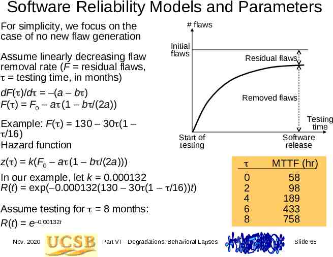
Software Reliability Models and Parameters For simplicity, we focus on the case of no new flaw generation Assume linearly decreasing flaw removal rate (F residual flaws, testing time, in months) # flaws Initial flaws dF( )/d –(a – b ) F( ) F0 – a (1 – b /(2a)) Example: F( ) 130 – 30 (1 – /16) Hazard function Removed flaws Testing time Software release Start of testing z( ) k(F0 – a (1 – b /(2a))) In our example, let k 0.000132 R(t) exp(–0.000132(130 – 30 (1 – /16))t) Assume testing for 8 months: R(t) e–0.00132t Nov. 2020 Residual flaws Part VI – Degradations: Behavioral Lapses 0 2 4 6 8 MTTF (hr) 58 98 189 433 758 Slide 65
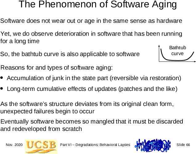
The Phenomenon of Software Aging Software does not wear out or age in the same sense as hardware Yet, we do observe deterioration in software that has been running for a long time So, the bathtub curve is also applicable to software Bathtub curve Reasons for and types of software aging: Accumulation of junk in the state part (reversible via restoration) Long-term cumulative effects of updates (patches and the like) As the software’s structure deviates from its original clean form, unexpected failures begin to occur Eventually software becomes so mangled that it must be discarded and redeveloped from scratch Nov. 2020 Part VI – Degradations: Behavioral Lapses Slide 66
More on Software Reliability Models Linearly decreasing flaw removal rate isn’t the only option in modeling Constant flaw removal rate has also been considered, but it does not lead to a very realistic model Exponentially decreasing flaw removal rate is more realistic than linearly decreasing, since flaw removal rate never really becomes 0 How does one go about estimating the model constants? Use handbook: public ones, or compiled from in-house data Match moments (mean, 2nd moment, . . .) to flaw removal data Least-squares estimation, particularly with multiple data sets Maximum-likelihood estimation (a statistical method) Nov. 2020 Part VI – Degradations: Behavioral Lapses Slide 67
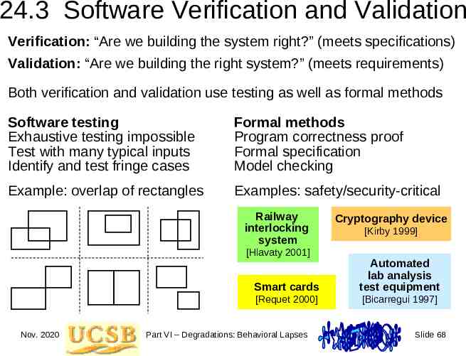
24.3 Software Verification and Validation Verification: “Are we building the system right?” (meets specifications) Validation: “Are we building the right system?” (meets requirements) Both verification and validation use testing as well as formal methods Software testing Exhaustive testing impossible Test with many typical inputs Identify and test fringe cases Formal methods Program correctness proof Formal specification Model checking Example: overlap of rectangles Examples: safety/security-critical Railway interlocking system [Hlavaty 2001] Nov. 2020 Cryptography device [Kirby 1999] Smart cards Automated lab analysis test equipment [Requet 2000] [Bicarregui 1997] Part VI – Degradations: Behavioral Lapses Slide 68
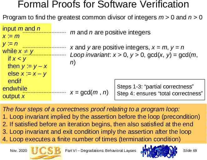
Formal Proofs for Software Verification Program to find the greatest common divisor of integers m 0 and n 0 input m and n x : m y : n while x y if x y then y : y – x else x : x – y endif endwhile output x m and n are positive integers x and y are positive integers, x m, y n Loop invariant: x 0, y 0, gcd(x, y) gcd(m, n) x gcd(m , n) Steps 1-3: “partial correctness” Step 4: ensures “total correctness” The four steps of a correctness proof relating to a program loop: 1. Loop invariant implied by the assertion before the loop (precondition) 2. If satisfied before an iteration begins, then also satisfied at the end 3. Loop invariant and exit condition imply the assertion after the loop 4. Loop executes a finite number of times (termination condition) Nov. 2020 Part VI – Degradations: Behavioral Lapses Slide 69
Software Flaw Tolerance Flaw avoidance strategies include (structured) design methodologies, software reuse, and formal methods Given that a complex piece of software will contain bugs, can we use redundancy to reduce the probability of software-induced failures? The ideas of masking redundancy, standby redundancy, and self-checking design have been shown to be applicable to software, leading to various types of fault-tolerant software “Flaw tolerance” is a better term; “fault tolerance” has been overused Masking redundancy: N-version programming Standby redundancy: the recovery-block scheme Self-checking design: N-self-checking programming Sources: Software Fault Tolerance, ed. by Michael R. Lyu, Wiley, 2005 (on-line book at http://www.cse.cuhk.edu.hk/ lyu/book/sft/index.html) Also, “Software Fault Tolerance: A Tutorial,” 2000 (NASA report, available on-line) Nov. 2020 Part VI – Degradations: Behavioral Lapses Slide 70
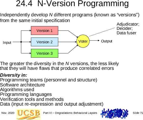
24.4 N-Version Programming Independently develop N different programs (known as “versions”) from the same initial specification Adjudicator; Decider; Data fuser Version 1 Input Version 2 Voter Output Version 3 The greater the diversity in the N versions, the less likely that they will have flaws that produce correlated errors Diversity in: Programming teams (personnel and structure) Software architecture Algorithms used Programming languages Verification tools and methods Data (input re-expression and output adjustment) Nov. 2020 Part VI – Degradations: Behavioral Lapses Slide 71
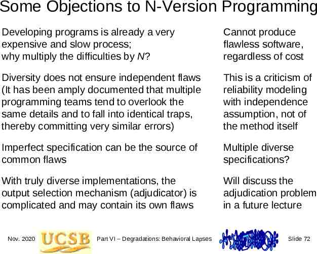
Some Objections to N-Version Programming Developing programs is already a very expensive and slow process; why multiply the difficulties by N? Cannot produce flawless software, regardless of cost Diversity does not ensure independent flaws (It has been amply documented that multiple programming teams tend to overlook the same details and to fall into identical traps, thereby committing very similar errors) This is a criticism of reliability modeling with independence assumption, not of the method itself Imperfect specification can be the source of common flaws Multiple diverse specifications? With truly diverse implementations, the output selection mechanism (adjudicator) is complicated and may contain its own flaws Will discuss the adjudication problem in a future lecture Nov. 2020 Part VI – Degradations: Behavioral Lapses Slide 72
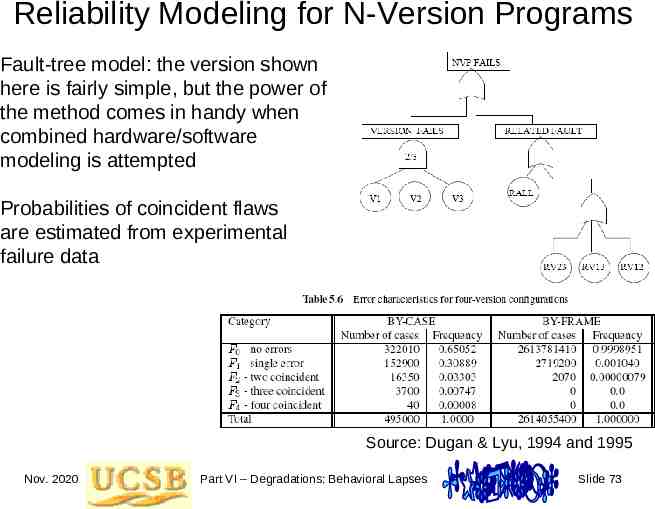
Reliability Modeling for N-Version Programs Fault-tree model: the version shown here is fairly simple, but the power of the method comes in handy when combined hardware/software modeling is attempted Probabilities of coincident flaws are estimated from experimental failure data Source: Dugan & Lyu, 1994 and 1995 Nov. 2020 Part VI – Degradations: Behavioral Lapses Slide 73
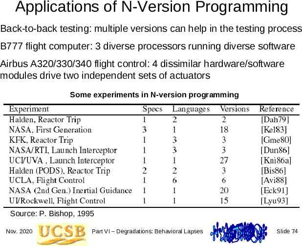
Applications of N-Version Programming Back-to-back testing: multiple versions can help in the testing process B777 flight computer: 3 diverse processors running diverse software Airbus A320/330/340 flight control: 4 dissimilar hardware/software modules drive two independent sets of actuators Some experiments in N-version programming Source: P. Bishop, 1995 Nov. 2020 Part VI – Degradations: Behavioral Lapses Slide 74
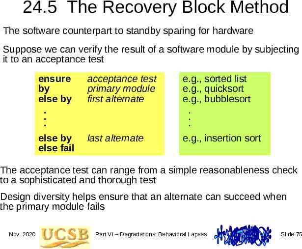
24.5 The Recovery Block Method The software counterpart to standby sparing for hardware Suppose we can verify the result of a software module by subjecting it to an acceptance test ensure by else by . . . acceptance test primary module first alternate e.g., sorted list e.g., quicksort e.g., bubblesort . . . else by else fail last alternate e.g., insertion sort The acceptance test can range from a simple reasonableness check to a sophisticated and thorough test Design diversity helps ensure that an alternate can succeed when the primary module fails Nov. 2020 Part VI – Degradations: Behavioral Lapses Slide 75
The Acceptance Test Problem Design of acceptance tests (ATs) that are both simple and thorough is very difficult; for example, to check the result of sorting, it is not enough to verify that the output sequence is monotonic Simplicity is desirable because acceptance test is executed after the primary computation, thus lengthening the critical path Thoroughness ensures that an incorrect result does not pass the test (of course, a correct result always passes a properly designed test) Some computations do have simple tests (inverse computation) Examples: square-rooting can be checked through squaring, and roots of a polynomial can be verified via polynomial evaluation At worst, the acceptance test might be as complex as the primary computation itself Nov. 2020 Part VI – Degradations: Behavioral Lapses Slide 76
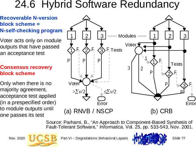
24.6 Hybrid Software Redundancy Recoverable N-version block scheme N-self-checking program Voter acts only on module outputs that have passed an acceptance test 1 1 F P 2 2 F P 3 3 F Tests 1 3 Voter v/2 2 3 Voter P Consensus recovery block scheme Only when there is no majority agreement, acceptance test applied (in a prespecified order) to module outputs until one passes its test 1 Modules 2 1 F P Tests 2 F P 3 F P v/2 Error (a) RNVB / NSCP Error (b) CRB Source: Parhami, B., “An Approach to Component-Based Synthesis of Fault-Tolerant Software,” Informatica, Vol. 25, pp. 533-543, Nov. 2001. Nov. 2020 Part VI – Degradations: Behavioral Lapses Slide 77
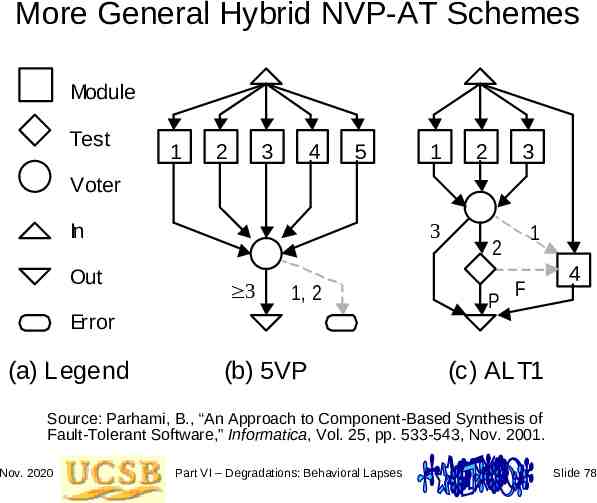
More General Hybrid NVP-AT Schemes Module Test 1 2 3 4 5 1 2 3 Voter In Out 3 3 1, 2 Error (a) Legend (b) 5VP 1 2 P F 4 (c) ALT1 Source: Parhami, B., “An Approach to Component-Based Synthesis of Fault-Tolerant Software,” Informatica, Vol. 25, pp. 533-543, Nov. 2001. Nov. 2020 Part VI – Degradations: Behavioral Lapses Slide 78