Chapter 9: Basics of Hypothesis Testing Mar 20, 2023

Chapter 9: Basics of Hypothesis Testing Mar 20, 2023

In Chapter 9: 9.1 Null and Alternative Hypotheses 9.2 Test Statistic 9.3 P-Value 9.4 Significance Level 9.5 One-Sample z Test 9.6 Power and Sample Size

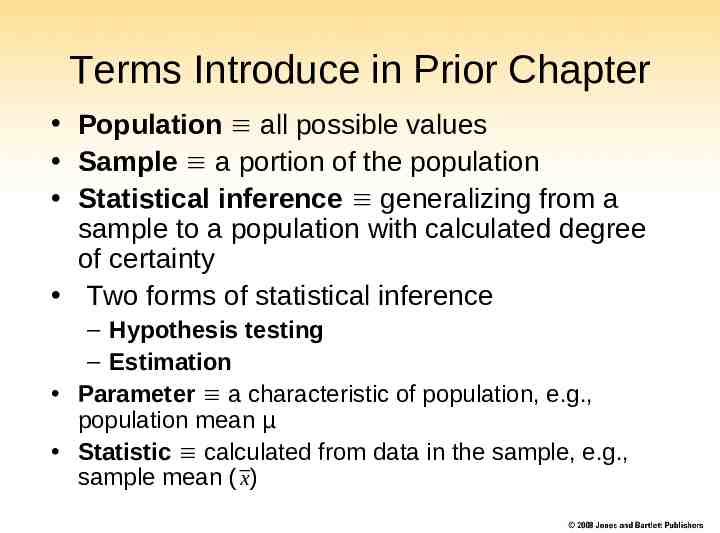
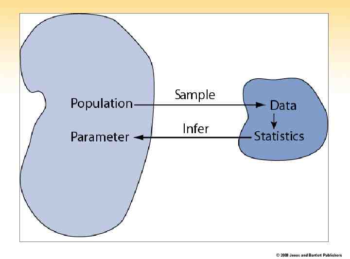
Terms Introduce in Prior Chapter Population all possible values Sample a portion of the population Statistical inference generalizing from a sample to a population with calculated degree of certainty Two forms of statistical inference – Hypothesis testing – Estimation Parameter a characteristic of population, e.g., population mean µ Statistic calculated from data in the sample, e.g., sample mean ( x )

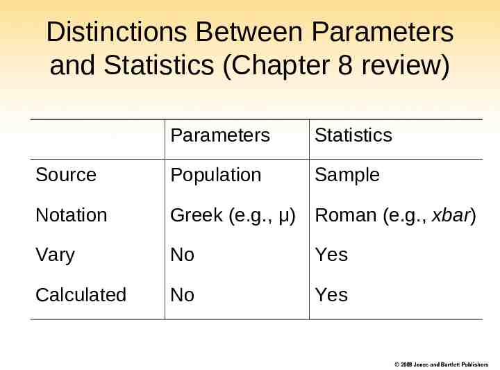
Distinctions Between Parameters and Statistics (Chapter 8 review) Parameters Statistics Source Population Sample Notation Greek (e.g., μ) Roman (e.g., xbar) Vary No Yes Calculated No Yes

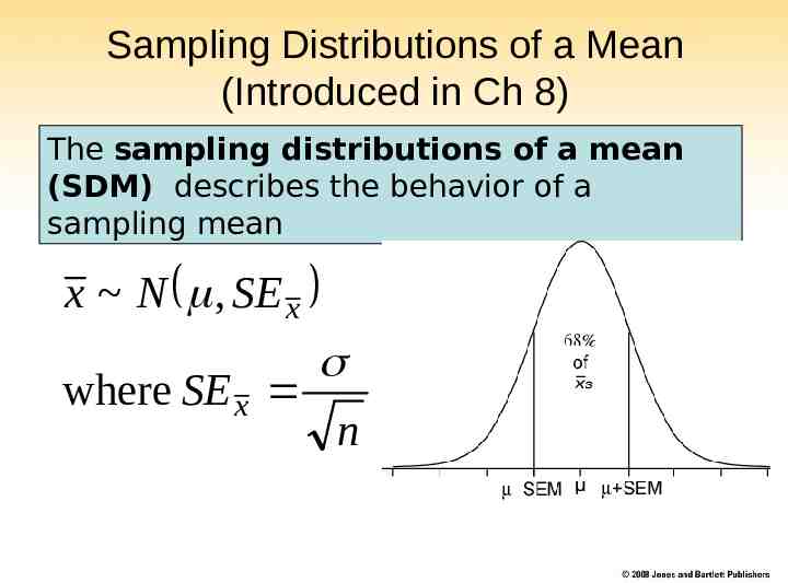
Sampling Distributions of a Mean (Introduced in Ch 8) The sampling distributions of a mean (SDM) describes the behavior of a sampling mean x N , SE x where SE x n

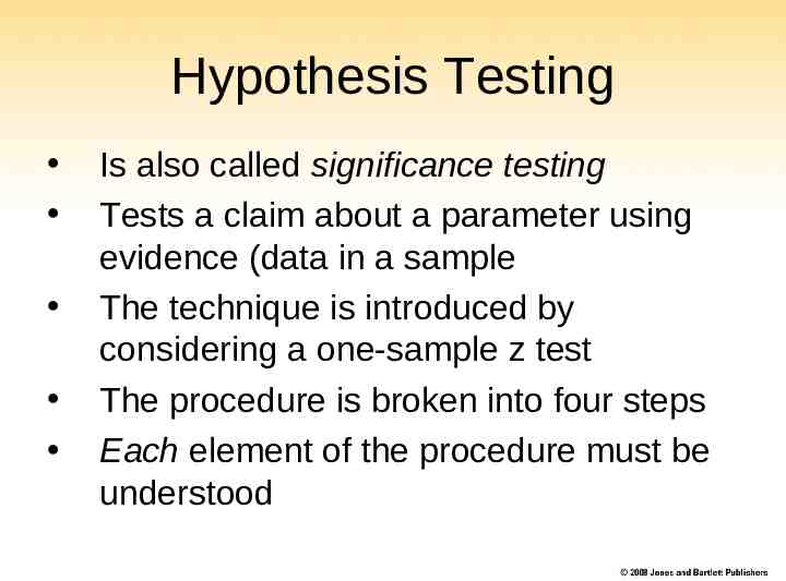
Hypothesis Testing Is also called significance testing Tests a claim about a parameter using evidence (data in a sample The technique is introduced by considering a one-sample z test The procedure is broken into four steps Each element of the procedure must be understood

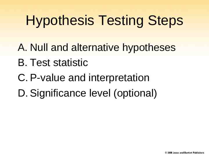
Hypothesis Testing Steps A. Null and alternative hypotheses B. Test statistic C. P-value and interpretation D. Significance level (optional)

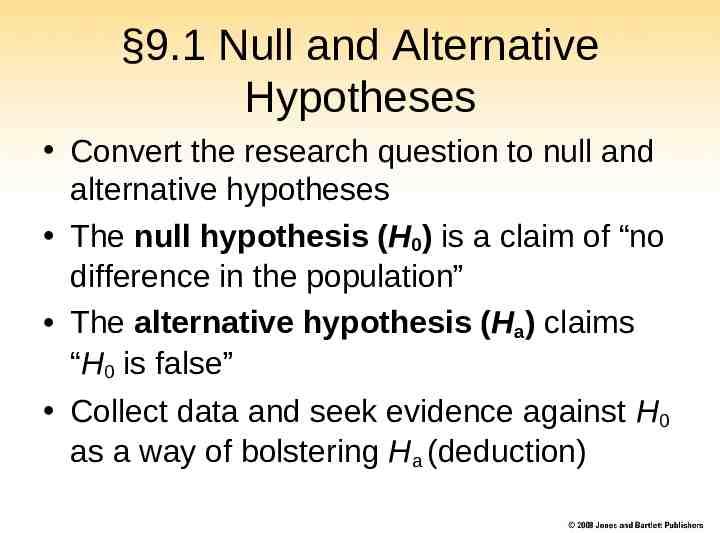
§9.1 Null and Alternative Hypotheses Convert the research question to null and alternative hypotheses The null hypothesis (H0) is a claim of “no difference in the population” The alternative hypothesis (Ha) claims “H0 is false” Collect data and seek evidence against H0 as a way of bolstering Ha (deduction)

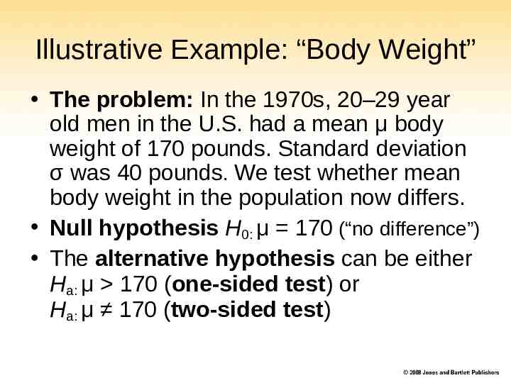
Illustrative Example: “Body Weight” The problem: In the 1970s, 20–29 year old men in the U.S. had a mean μ body weight of 170 pounds. Standard deviation σ was 40 pounds. We test whether mean body weight in the population now differs. Null hypothesis H0: μ 170 (“no difference”) The alternative hypothesis can be either Ha: μ 170 (one-sided test) or Ha: μ 170 (two-sided test)

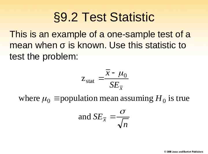
§9.2 Test Statistic This is an example of a one-sample test of a mean when σ is known. Use this statistic to test the problem: z stat x 0 SE x where 0 population mean assuming H 0 is true and SE x n

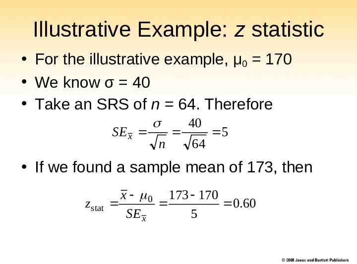
Illustrative Example: z statistic For the illustrative example, μ0 170 We know σ 40 Take an SRS of n 64. Therefore SE x n 40 64 5 If we found a sample mean of 173, then z stat x 0 173 170 0.60 SE x 5

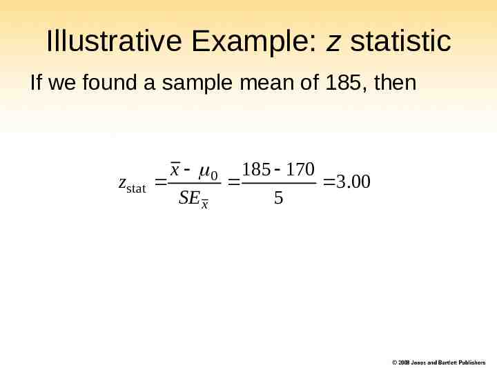
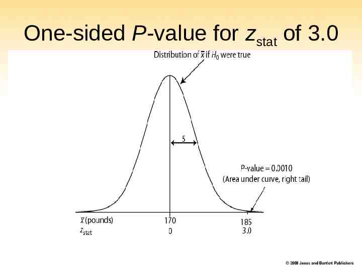
Illustrative Example: z statistic If we found a sample mean of 185, then zstat x 0 185 170 3.00 SE x 5

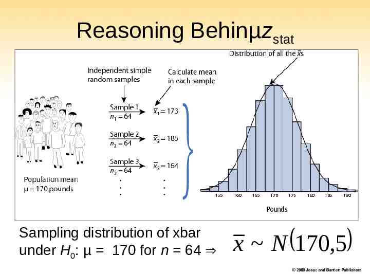
Reasoning Behinµzstat Sampling distribution of xbar under H0: µ 170 for n 64 x N 170,5

§9.3 P-value The P-value answer the question: What is the probability of the observed test statistic or one more extreme when H0 is true? This corresponds to the AUC in the tail of the Standard Normal distribution beyond the zstat. Convert z statistics to P-value : For Ha: μ μ0 P Pr(Z zstat) right-tail beyond zstat For Ha: μ μ0 P Pr(Z zstat) left tail beyond zstat For Ha: μ μ0 P 2 one-tailed P-value Use Table B or software to find these probabilities (next two slides).

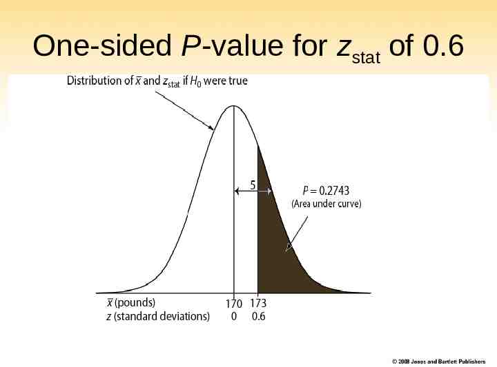
One-sided P-value for zstat of 0.6

One-sided P-value for zstat of 3.0

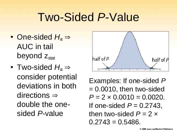
Two-Sided P-Value One-sided Ha AUC in tail beyond zstat Two-sided Ha consider potential deviations in both directions double the onesided P-value Examples: If one-sided P 0.0010, then two-sided P 2 0.0010 0.0020. If one-sided P 0.2743, then two-sided P 2 0.2743 0.5486.

Interpretation P-value answer the question: What is the probability of the observed test statistic when H0 is true? Thus, smaller and smaller P-values provide stronger and stronger evidence against H0 Small P-value strong evidence

Interpretation Conventions* P 0.10 non-significant evidence against H0 0.05 P 0.10 marginally significant evidence 0.01 P 0.05 significant evidence against H0 P 0.01 highly significant evidence against H0 Examples P .27 non-significant evidence against H0 P .01 highly significant evidence against H0 * It is unwise to draw firm borders for “significance”

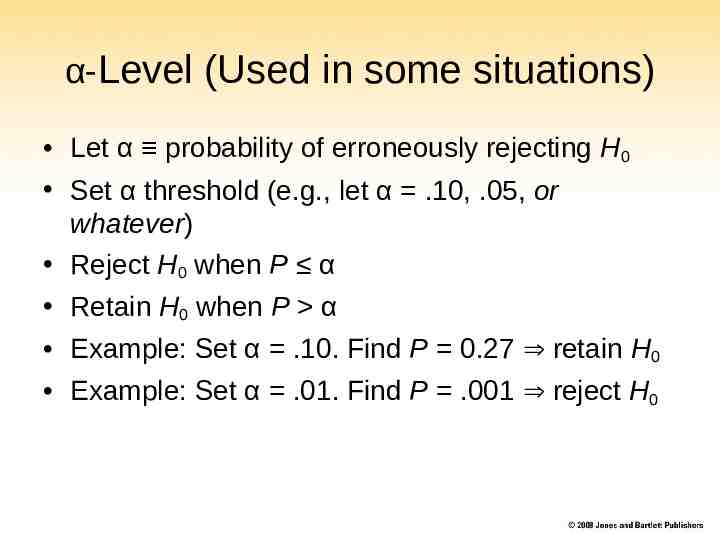
α-Level (Used in some situations) Let α probability of erroneously rejecting H0 Set α threshold (e.g., let α .10, .05, or whatever) Reject H0 when P α Retain H0 when P α Example: Set α .10. Find P 0.27 retain H0 Example: Set α .01. Find P .001 reject H0

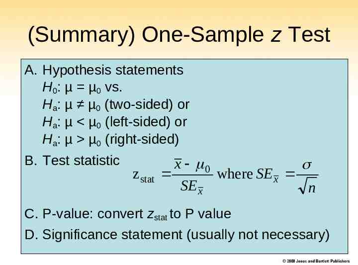
(Summary) One-Sample z Test A. Hypothesis statements H0: µ µ0 vs. Ha: µ µ0 (two-sided) or Ha: µ µ0 (left-sided) or Ha: µ µ0 (right-sided) B. Test statistic z stat x 0 where SE x SE x n C. P-value: convert zstat to P value D. Significance statement (usually not necessary)

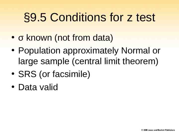
§9.5 Conditions for z test σ known (not from data) Population approximately Normal or large sample (central limit theorem) SRS (or facsimile) Data valid

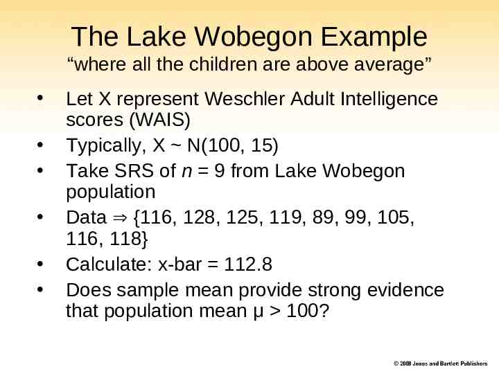
The Lake Wobegon Example “where all the children are above average” Let X represent Weschler Adult Intelligence scores (WAIS) Typically, X N(100, 15) Take SRS of n 9 from Lake Wobegon population Data {116, 128, 125, 119, 89, 99, 105, 116, 118} Calculate: x-bar 112.8 Does sample mean provide strong evidence that population mean μ 100?

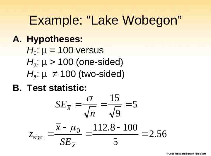
Example: “Lake Wobegon” A. Hypotheses: H0: µ 100 versus Ha: µ 100 (one-sided) Ha: µ 100 (two-sided) B. Test statistic: z stat 15 SE x 5 n 9 x 0 112.8 100 2.56 SE x 5

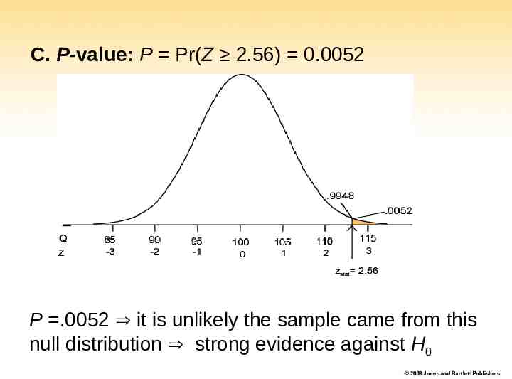
C. P-value: P Pr(Z 2.56) 0.0052 P .0052 it is unlikely the sample came from this null distribution strong evidence against H0

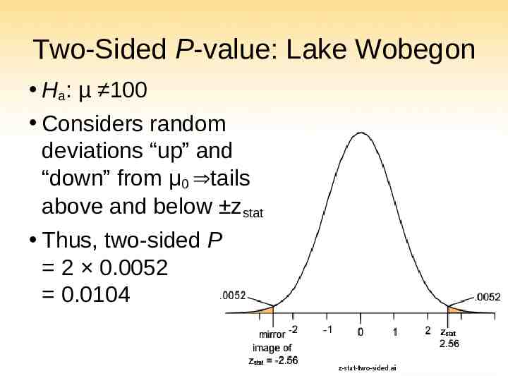
Two-Sided P-value: Lake Wobegon Ha: µ 100 Considers random deviations “up” and “down” from μ0 tails above and below zstat Thus, two-sided P 2 0.0052 0.0104

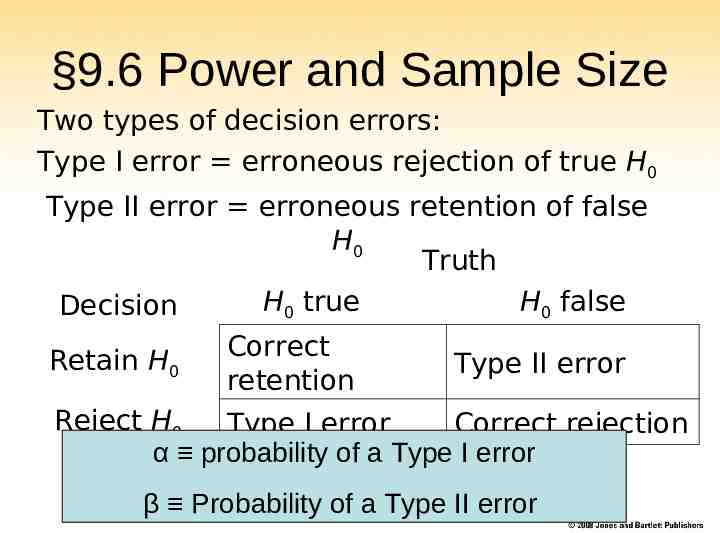
§9.6 Power and Sample Size Two types of decision errors: Type I error erroneous rejection of true H0 Type II error erroneous retention of false H0 Truth H0 true H0 false Decision Retain H0 Correct retention Type II error Reject H0 Type I error Correct rejection α probability of a Type I error β Probability of a Type II error

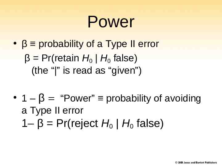
Power β probability of a Type II error β Pr(retain H0 H0 false) (the “ ” is read as “given”) 1 – β “Power” probability of avoiding a Type II error 1– β Pr(reject H0 H0 false)

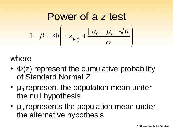
Power of a z test 0 a n 1 z1 2 where Φ(z) represent the cumulative probability of Standard Normal Z μ0 represent the population mean under the null hypothesis μa represents the population mean under the alternative hypothesis

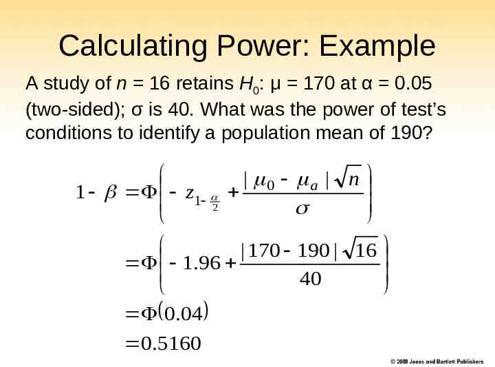
Calculating Power: Example A study of n 16 retains H0: μ 170 at α 0.05 (two-sided); σ is 40. What was the power of test’s conditions to identify a population mean of 190? n a 1 z1 0 2 170 190 16 1.96 40 0.04 0.5160

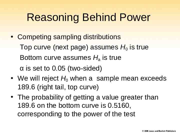
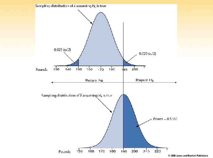
Reasoning Behind Power Competing sampling distributions Top curve (next page) assumes H0 is true Bottom curve assumes Ha is true α is set to 0.05 (two-sided) We will reject H0 when a sample mean exceeds 189.6 (right tail, top curve) The probability of getting a value greater than 189.6 on the bottom curve is 0.5160, corresponding to the power of the test

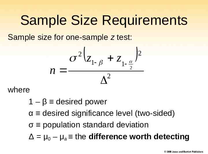
Sample Size Requirements Sample size for one-sample z test: 2 n z1 z1 2 2 2 where 1 – β desired power α desired significance level (two-sided) σ population standard deviation Δ μ0 – μa the difference worth detecting

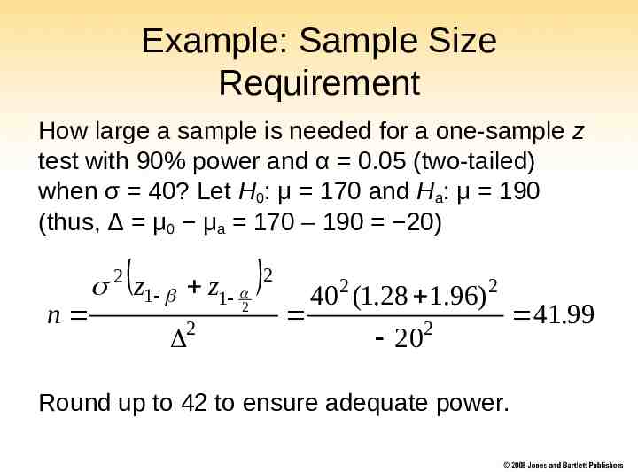
Example: Sample Size Requirement How large a sample is needed for a one-sample z test with 90% power and α 0.05 (two-tailed) when σ 40? Let H0: μ 170 and Ha: μ 190 (thus, Δ μ0 μa 170 – 190 20) 2 n z1 z1 2 2 2 2 40 (1.28 1.96) 20 2 2 Round up to 42 to ensure adequate power. 41.99

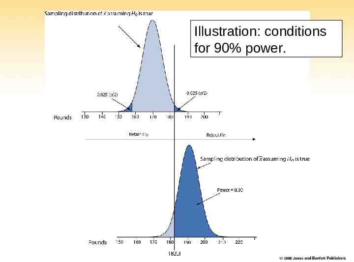
Illustration: conditions for 90% power.