Chapter 2: An Introduction to Linear Programming Instructor: Dr.
46 Slides2.08 MB
Chapter 2: An Introduction to Linear Programming Instructor: Dr. Mohamed Mostafa
Overview Linear Programming Problem Problem Formulation A Simple Maximization Problem Graphical Solution Procedure Extreme Points and the Optimal Solution A Simple Minimization Problem Special Cases 2
Linear Programming Linear programming has nothing to do with computer programming. The use of the word “programming” here means “choosing a course of action”. Linear programming is a problem-solving approach developed to help managers make decisions.
Linear Programming (LP) Problem The maximization or minimization of some quantity is the objective in all linear programming problems. All LP problems have – Constraints that limit the objective function value. – feasible solution satisfies all the problem's constraints. – optimal solution is the largest possible objective function value when maximizing (or smallest when minimizing). A graphical solution method can be used to solve a linear program with two variables.
Linear Programming (LP) Problem If both the objective function and the constraints are linear, the problem is referred to as a linear programming problem. Linear functions are functions in which each variable appears in a separate term raised to the first power and is multiplied by a constant (which could be 0). Linear constraints are linear functions that are restricted to be "less than or equal to", "equal to", or "greater than or equal to" a constant.
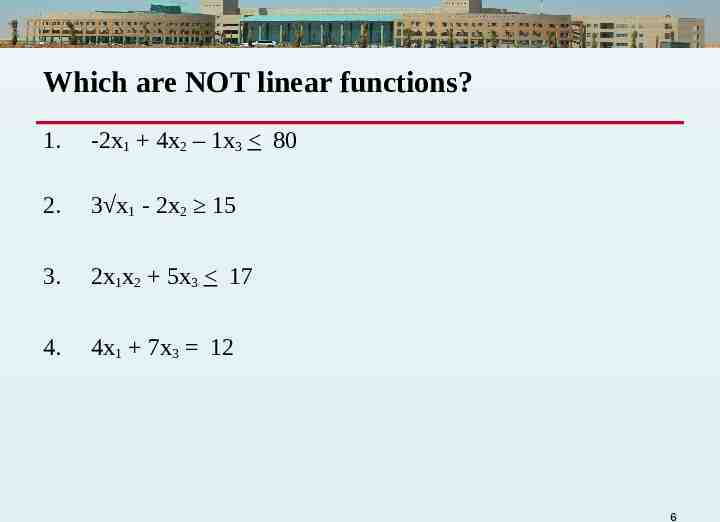
Which are NOT linear functions? 1. -2x1 4x2 – 1x3 80 2. 3 x1 - 2x2 15 3. 2x1x2 5x3 17 4. 4x1 7x3 12 6
Problem Formulation Problem formulation or modeling is the process of translating a verbal statement of a problem into a mathematical statement. Formulating models is an art that can only be mastered with practice and experience. Every LP problem has some unique features, but most problems also have common features. General guidelines for LP model formulation are illustrated on the slides that follow.
Guidelines for Model Formulation Read and Understand the problem. Describe the objective. Describe each constraint. Define the decision variables. Write the objective in terms of the decision variables. Write the constraints in terms of the decision variables.
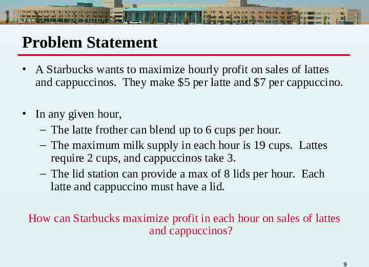
Problem Statement A Starbucks wants to maximize hourly profit on sales of lattes and cappuccinos. They make 5 per latte and 7 per cappuccino. In any given hour, – The latte frother can blend up to 6 cups per hour. – The maximum milk supply in each hour is 19 cups. Lattes require 2 cups, and cappuccinos take 3. – The lid station can provide a max of 8 lids per hour. Each latte and cappuccino must have a lid. How can Starbucks maximize profit in each hour on sales of lattes and cappuccinos? 9
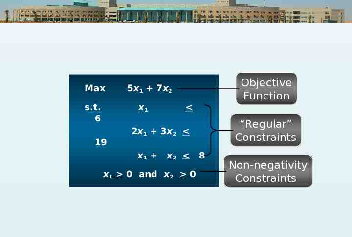
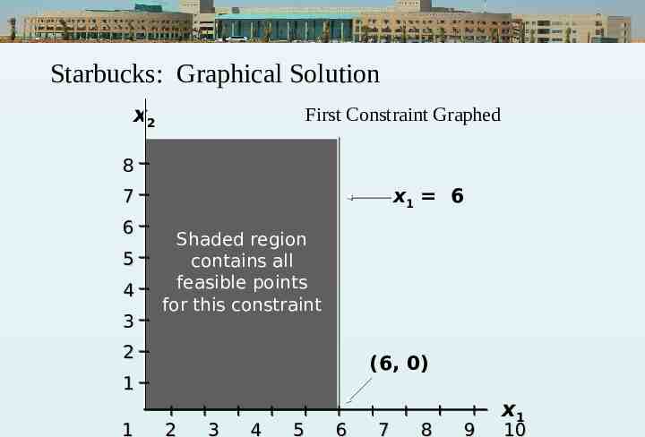
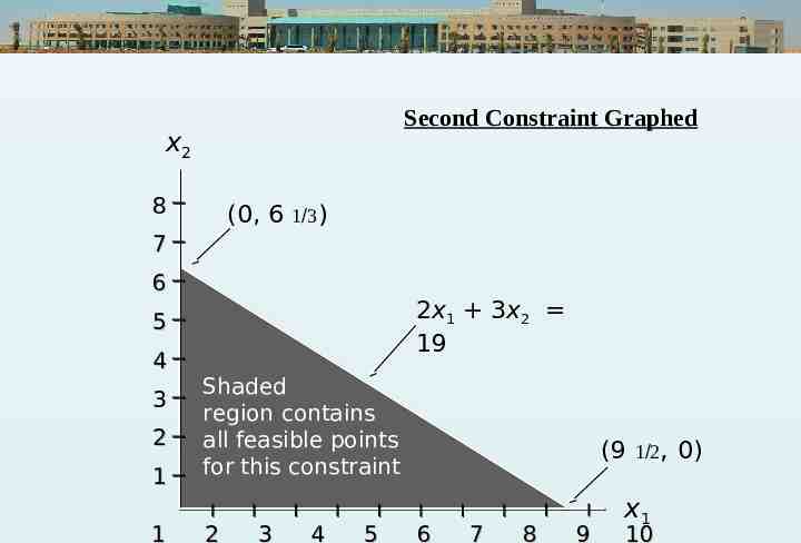
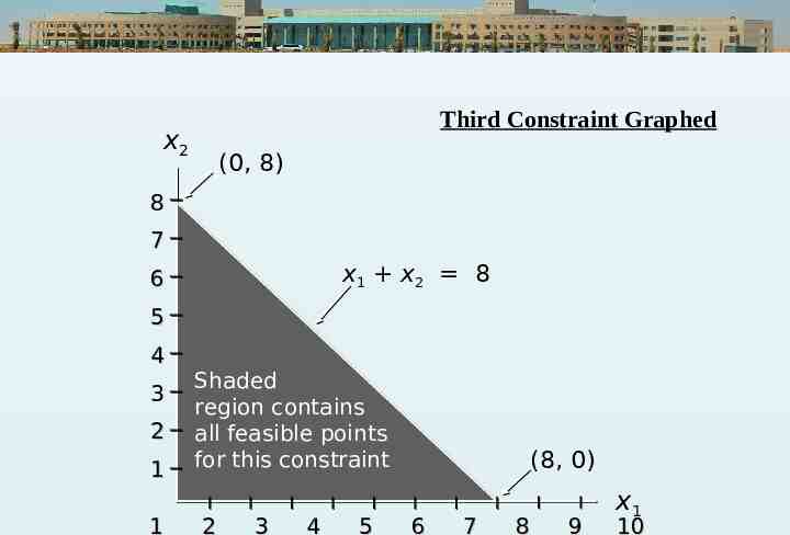
Max s.t. 6 Objective Function 5x1 7x2 x1 “Regular” Constraints 2x1 3x2 19 x1 x2 x1 0 and x2 0 8 Non-negativity Constraints
Graphical Solution Prepare a graph of the feasible solutions for each of the constraints. Determine the feasible region that satisfies all the constraints simultaneously. Type of constraint Feasible region (usually) will be – above/to the right – below/to the left – the line Draw an objective function line. Move parallel objective function lines toward larger objective function values without entirely leaving the feasible region. Any feasible solution on the objective function line with the largest value is an optimal solution. 11
Starbucks: Graphical Solution x2 8 7 6 5 4 3 2 1 1 2 3 4 5 6 7 8 9 x1 10
Starbucks: Graphical Solution x2 First Constraint Graphed 8 x1 6 7 6 5 4 3 Shaded region contains all feasible points for this constraint 2 (6, 0) 1 1 2 3 4 5 6 7 8 9 x1 10
Second Constraint Graphed x2 8 (0, 6 ) 7 6 2x1 3x2 19 5 4 3 2 1 1 Shaded region contains all feasible points for this constraint 2 3 4 5 (9 , 0) 6 7 8 9 x1 10
Third Constraint Graphed x2 (0, 8) 8 7 x1 x2 8 6 5 4 3 2 1 1 Shaded region contains all feasible points for this constraint 2 3 4 5 (8, 0) 6 7 8 9 x1 10
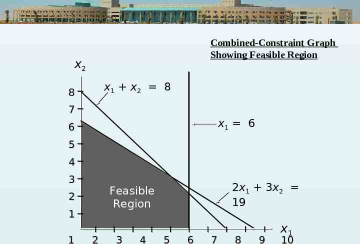
Combined-Constraint Graph Showing Feasible Region x2 x1 x2 8 8 7 x1 6 6 5 4 3 2 1 1 2x1 3x2 19 Feasible Region 2 3 4 5 6 7 8 9 x1 10
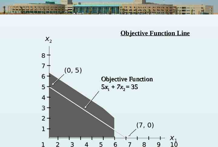
Objective Function Line x2 8 7 (0, 5) 6 Objective Function 5x1 7x2 35 5 4 3 2 (7, 0) 1 1 2 3 4 5 6 7 8 9 x1 10
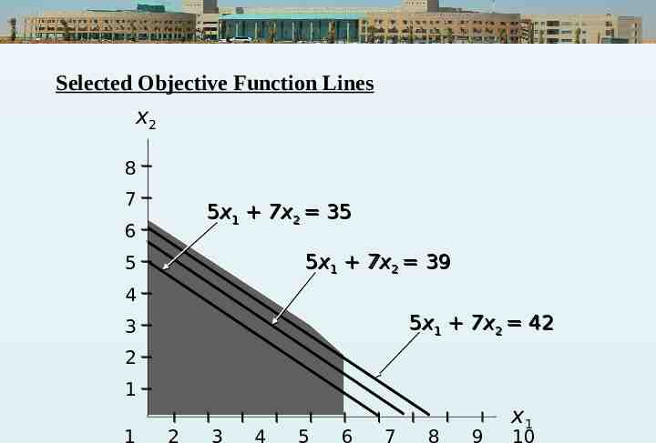
Selected Objective Function Lines x2 8 7 5x1 7x2 35 6 5x1 7x2 39 5 4 5x1 7x2 42 3 2 1 1 2 3 4 5 6 7 8 9 x1 10
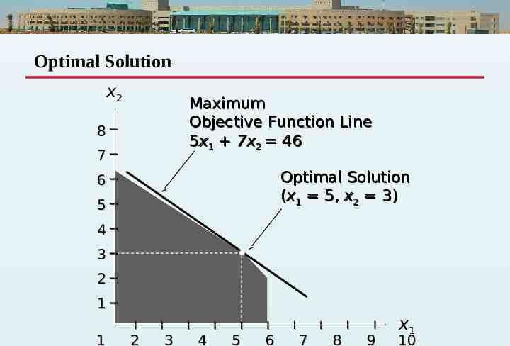
Optimal Solution x2 Maximum Objective Function Line 5x1 7x2 46 8 7 Optimal Solution (x1 5, x2 3) 6 5 4 3 2 1 1 2 3 4 5 6 7 8 9 x1 10
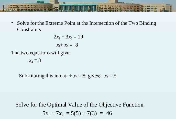
Solve for the Extreme Point at the Intersection of the Two Binding Constraints 2x1 3x2 19 x 1 x 2 8 The two equations will give: x2 3 Substituting this into x1 x2 8 gives: x1 5 Solve for the Optimal Value of the Objective Function 5x1 7x2 5(5) 7(3) 46
Extreme Points and the Optimal Solution The corners or vertices of the feasible region are referred to as the extreme points. An optimal solution to an LP problem can be found at an extreme point of the feasible region. When looking for the optimal solution, you do not have to evaluate all feasible solution points; consider only the extreme points of the feasible region.
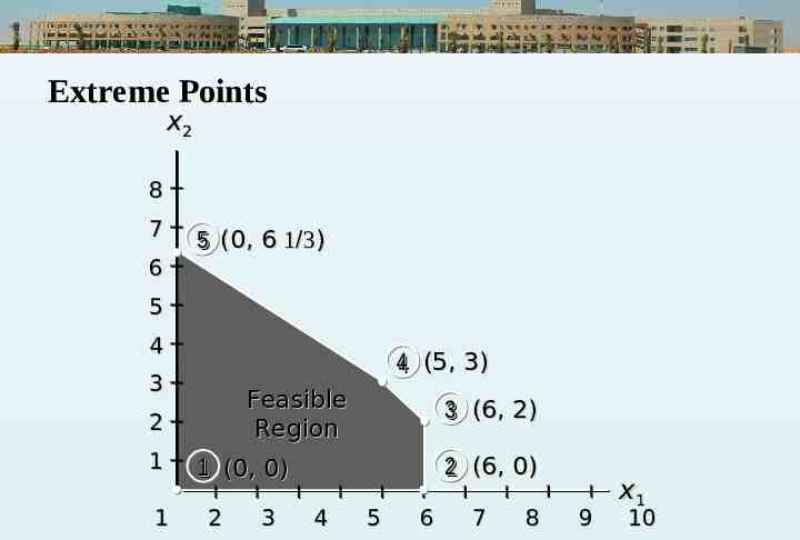
Extreme Points x2 8 7 6 5 (0, 6 ) 5 4 4 (5, 3) 3 Feasible Region 2 1 1 3 (6, 2) 2 (6, 0) 1 (0, 0) 2 3 4 5 6 7 8 9 x1 10
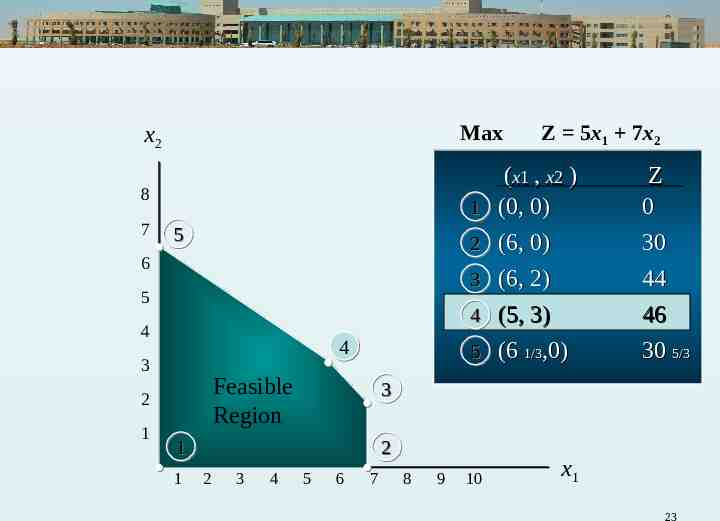
Max x2 8 7 10 x1 2 6 3 5 4 4 4 3 Feasible Region 2 1 5 (x1 , x2 ) (0, 0) (6, 0) (6, 2) (5, 3) (6 1/3,0) 1 5 2 2 3 4 Z 0 30 44 46 30 5/3 3 1 1 Z 5x1 7x2 5 6 7 8 9 23
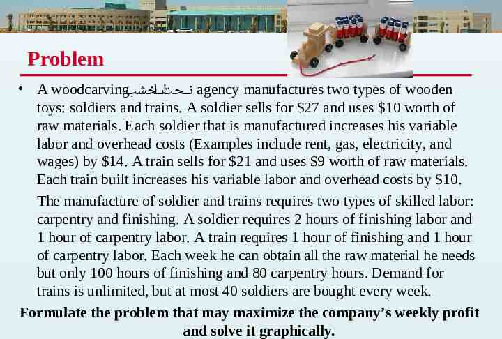
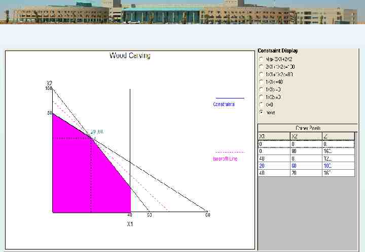
Problem A woodcarving ت لخشب ن ح ا agency manufactures two types of wooden toys: soldiers and trains. A soldier sells for 27 and uses 10 worth of raw materials. Each soldier that is manufactured increases his variable labor and overhead costs (Examples include rent, gas, electricity, and wages) by 14. A train sells for 21 and uses 9 worth of raw materials. Each train built increases his variable labor and overhead costs by 10. The manufacture of soldier and trains requires two types of skilled labor: carpentry and finishing. A soldier requires 2 hours of finishing labor and 1 hour of carpentry labor. A train requires 1 hour of finishing and 1 hour of carpentry labor. Each week he can obtain all the raw material he needs but only 100 hours of finishing and 80 carpentry hours. Demand for trains is unlimited, but at most 40 soldiers are bought every week. Formulate the problem that may maximize the company’s weekly profit and solve it graphically.
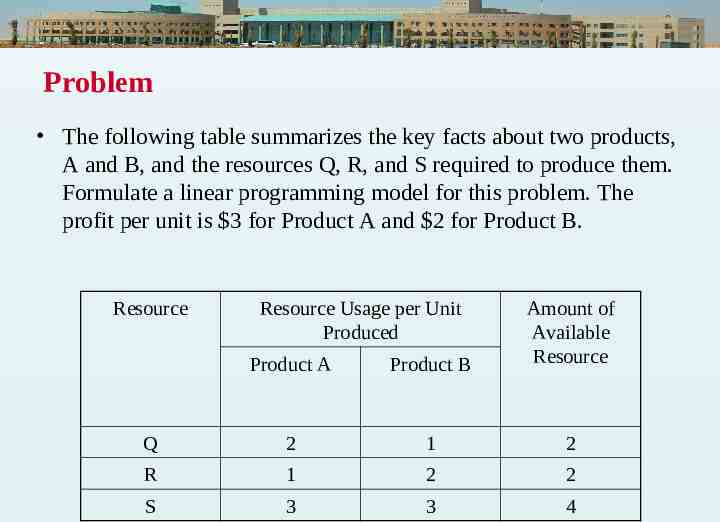
Problem The following table summarizes the key facts about two products, A and B, and the resources Q, R, and S required to produce them. Formulate a linear programming model for this problem. The profit per unit is 3 for Product A and 2 for Product B. Resource Resource Usage per Unit Produced Product A Product B Amount of Available Resource Q 2 1 2 R 1 2 2 S 3 3 4
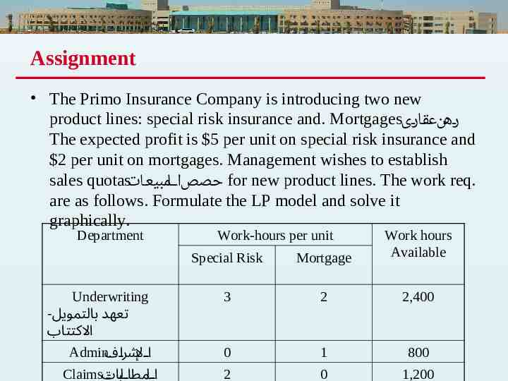
Assignment The Primo Insurance Company is introducing two new product lines: special risk insurance and. Mortgages رهنعقارى The expected profit is 5 per unit on special risk insurance and 2 per unit on mortgages. Management wishes to establish sales quotas حصصا لمبيعات for new product lines. The work req. are as follows. Formulate the LP model and solve it graphically. Department Work-hours per unit Special Risk Mortgage Work hours Available Underwriting - تعهد بالتمويل االكتتاب 3 2 2,400 Admin. ا إلشراف 0 1 800 Claims بات - ا لمطا ل 2 0 1,200
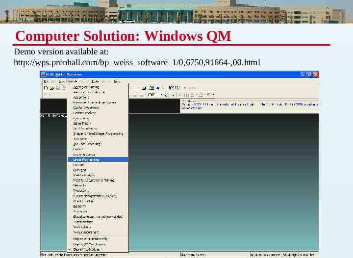
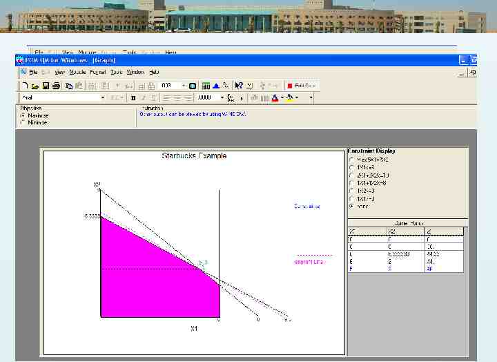
Computer Solution: Windows QM Demo version available at: http://wps.prenhall.com/bp weiss software 1/0,6750,91664-,00.html
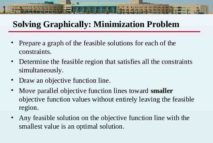
Solving Graphically: Minimization Problem Prepare a graph of the feasible solutions for each of the constraints. Determine the feasible region that satisfies all the constraints simultaneously. Draw an objective function line. Move parallel objective function lines toward smaller objective function values without entirely leaving the feasible region. Any feasible solution on the objective function line with the smallest value is an optimal solution.
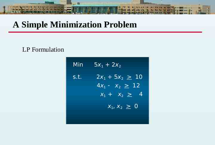
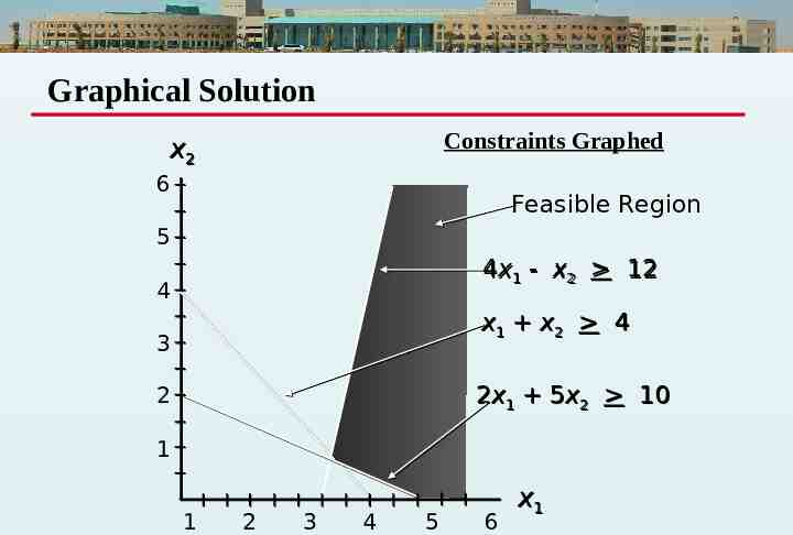
A Simple Minimization Problem LP Formulation Min s.t. 5x1 2x2 2x1 5x2 10 4x1 x2 12 x 1 x2 x 1, x 2 0 4
Graphical Solution Constraints Graphed x2 6 Feasible Region 5 4x1 x2 12 4 x1 x2 4 3 2x1 5x2 10 2 1 1 2 3 4 5 6 x1
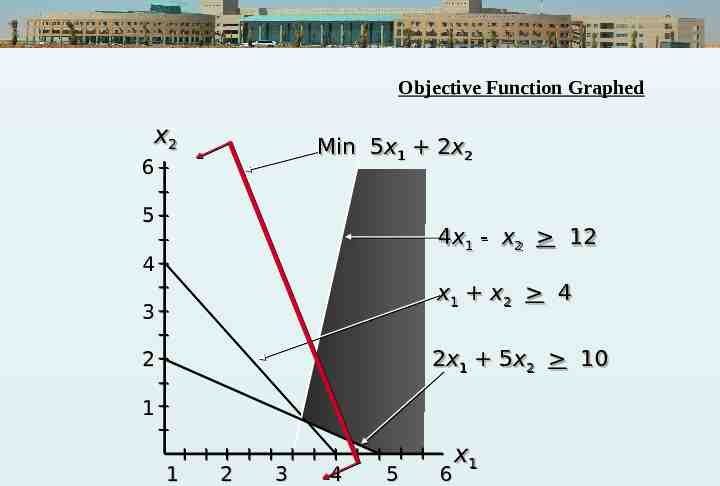
Objective Function Graphed x22 Min 5x11 2x22 6 5 4x11 x22 12 4 x11 x22 4 3 2x11 5x22 10 2 1 1 2 3 4 5 6 x11
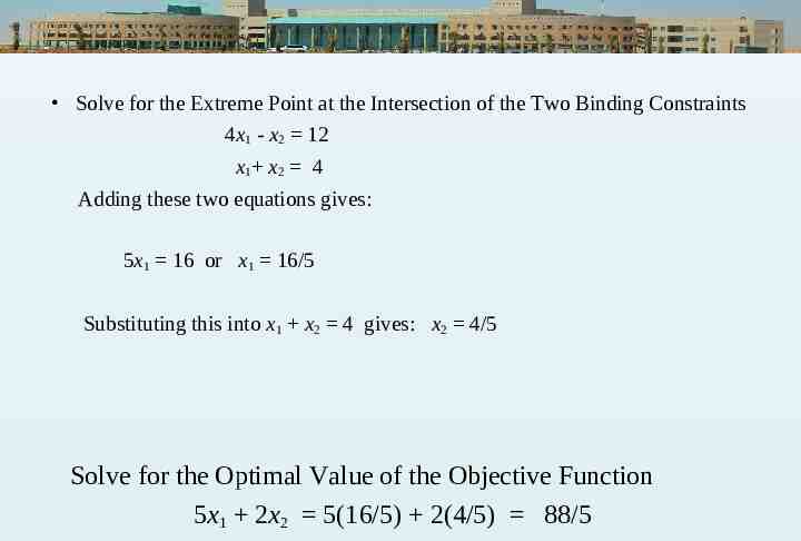
Solve for the Extreme Point at the Intersection of the Two Binding Constraints 4x1 - x2 12 x 1 x2 4 Adding these two equations gives: 5x1 16 or x1 16/5 Substituting this into x1 x2 4 gives: x2 4/5 Solve for the Optimal Value of the Objective Function 5x1 2x2 5(16/5) 2(4/5) 88/5
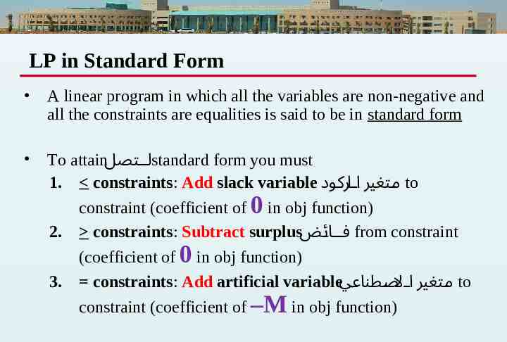
LP in Standard Form A linear program in which all the variables are non-negative and all the constraints are equalities is said to be in standard form To attain ل تصل standard form you must 1. constraints: Add slack variable متغير ا لركود to constraint (coefficient of 0 in obj function) 2. constraints: Subtract surplus ف ائض from constraint (coefficient of 0 in obj function) 3. constraints: Add artificial variable متغير ا الصطناعي to constraint (coefficient of –M in obj function)
Slack and surplus variables represent the difference between the left and right sides of the constraints. Slack is any unused resource, while surplus is the amount over some required minimum level. The objective function coefficient for slack and surplus variables is equal to 0. If slack/surplus variables are equal to 0 for a constraint, the constraint is said to be binding ُم لزِم .
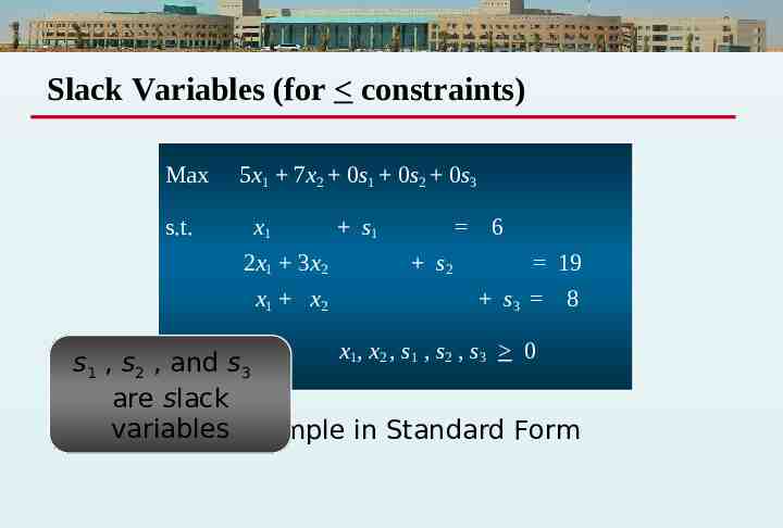
Slack Variables (for constraints) Max s.t. 5x1 7x2 0s1 0s2 0s3 x1 2x1 3x2 x1 x2 s1 s2 6 19 s3 8 x1, x2 , s1 , s2 , s3 0 s1 , s2 , and s3 are slack variables Example in Standard Form
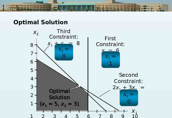
Optimal Solution Third Constraint: x1 x2 8 s3 0 x2 8 7 First Constraint: x1 6 s1 1 6 5 Second Constraint: 2x1 3x2 s19 2 0 4 3 2 1 1 Optimal Solution (x1 5, x2 3) 2 3 4 5 6 7 8 9 x1 10
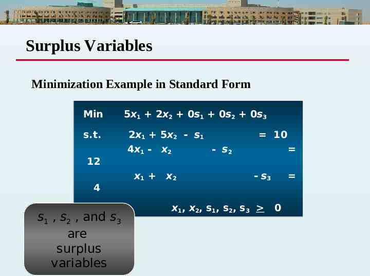
Surplus Variables Minimization Example in Standard Form Min s.t. 5x1 2x2 0s1 0s2 0s3 2x1 5x2 s1 4x1 x2 10 s2 12 x1 x2 s3 4 s1 , s2 , and s3 are surplus variables x1, x2, s1, s2, s3 0
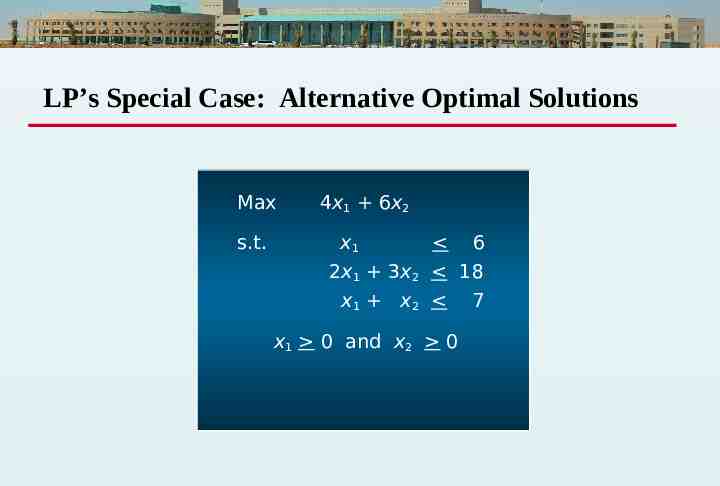
LP’s Special Case: Alternative Optimal Solutions Max s.t. 4x1 6x2 x1 6 2x1 3x2 18 x1 x2 x1 0 and x2 0 7
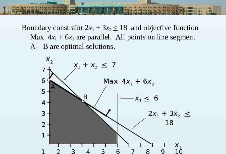
Boundary constraint 2x1 3x2 18 and objective function Max 4x1 6x2 are parallel. All points on line segment A – B are optimal solutions. x2 x1 x2 7 7 6 5 Max 4x1 6x2 A B 4 x1 6 2x1 3x2 18 3 2 1 1 2 3 4 5 6 7 8 9 x1 10
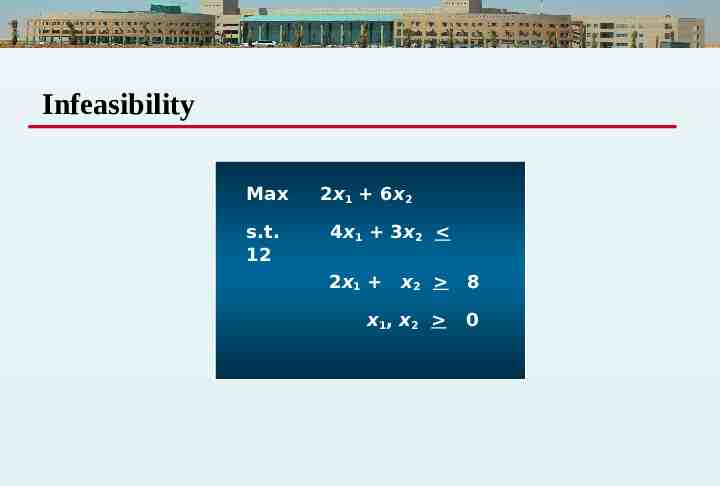
Infeasibility Max s.t. 12 2x1 6x2 4x1 3x2 2x1 x2 8 x1, x2 0
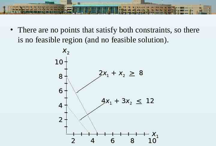
There are no points that satisfy both constraints, so there is no feasible region (and no feasible solution). x2 10 2x1 x2 8 8 6 4x1 3x2 12 4 2 2 4 6 8 x1 10
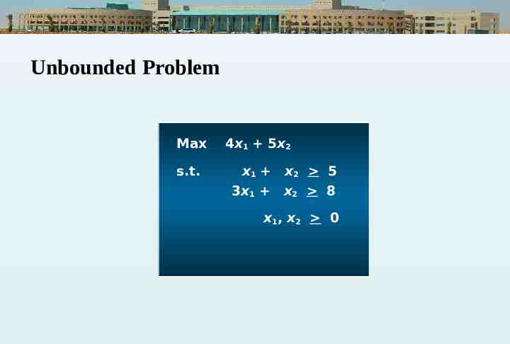
Unbounded Problem Max 4x1 5x2 s.t. x1 x2 5 3x1 x2 8 x1, x2 0
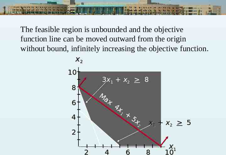
The feasible region is unbounded and the objective function line can be moved outward from the origin without bound, infinitely increasing the objective function. x2 10 3x1 x2 8 8 Ma x 6 4x 1 4 5x 2 x1 x2 5 2 2 4 6 8 x1 10
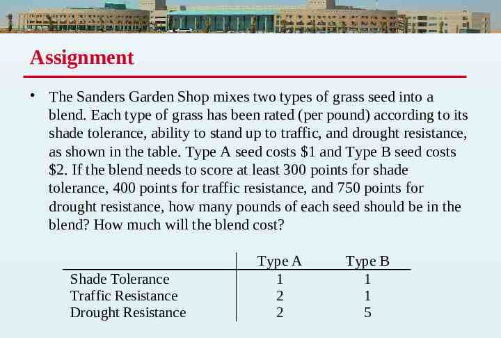
Assignment The Sanders Garden Shop mixes two types of grass seed into a blend. Each type of grass has been rated (per pound) according to its shade tolerance, ability to stand up to traffic, and drought resistance, as shown in the table. Type A seed costs 1 and Type B seed costs 2. If the blend needs to score at least 300 points for shade tolerance, 400 points for traffic resistance, and 750 points for drought resistance, how many pounds of each seed should be in the blend? How much will the blend cost? Shade Tolerance Traffic Resistance Drought Resistance Type A 1 2 2 Type B 1 1 5