Process Scheduling B.Ramamurthy Page 1 05/12/23
27 Slides924.50 KB
Process Scheduling B.Ramamurthy Page 1 05/12/23
Introduction An important aspect of multiprogramming is scheduling. The resources that are scheduled are IO and processors. The goal is to achieve – High processor utilization – High throughput number of processes completed per unit time – Low response time time elapse from the submission of a request to the beginning of the response Page 2 05/12/23
Topics for discussion Motivation Types of scheduling Short-term scheduling Various scheduling criteria Various algorithms – Priority queues – First-come, first-served – Round-robin – Shortest process first – Shortest remaining time and others Page 3 05/12/23
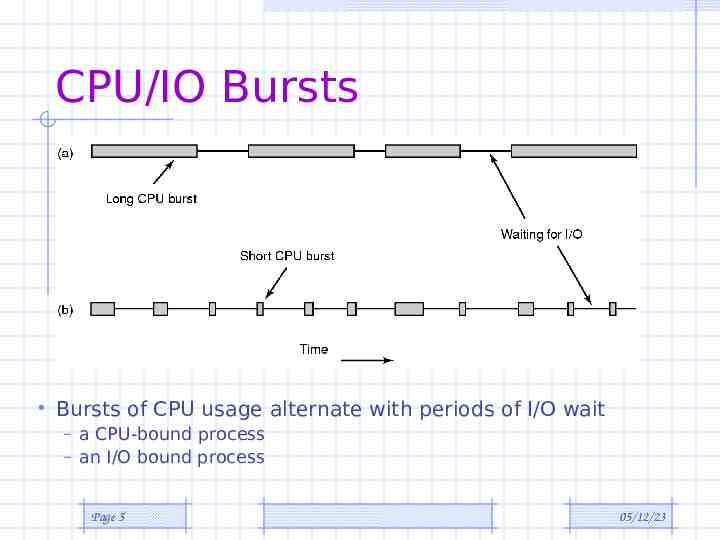
The CPU-I/O Cycle We observe that processes require alternate use of processor and I/O in a repetitive fashion Each cycle consist of a CPU burst (typically of 5 ms) followed by a (usually longer) I/O burst A process terminates on a CPU burst CPU-bound processes have longer CPU bursts than I/O-bound processes Page 4 05/12/23
CPU/IO Bursts Bursts of CPU usage alternate with periods of I/O wait – a CPU-bound process – an I/O bound process Page 5 05/12/23
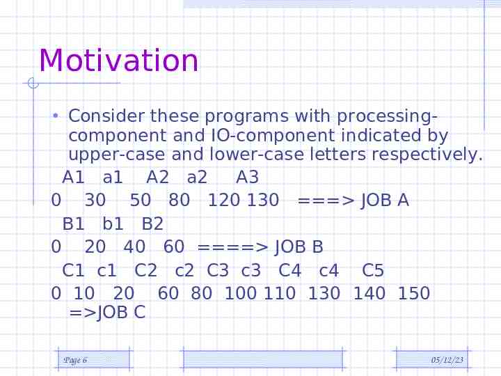
Motivation Consider these programs with processing- component and IO-component indicated by upper-case and lower-case letters respectively. A1 a1 A2 a2 A3 0 30 50 80 120 130 JOB A B1 b1 B2 0 20 40 60 JOB B C1 c1 C2 c2 C3 c3 C4 c4 C5 0 10 20 60 80 100 110 130 140 150 JOB C Page 6 05/12/23
Motivation The starting and ending time of each component are indicated beneath the symbolic references (A1, b1 etc.) Now lets consider three different ways for scheduling: no overlap, round-robin, simple overlap. Compare utilization U time CPU busy / total run time Page 7 05/12/23
Scheduling Criteria CPU utilization – keep the CPU as busy as possible Throughput – # of processes that complete their execution per time unit Turnaround time – amount of time to execute a particular process Waiting time – amount of time a process has been waiting in the ready queue and blocked queue Response time – amount of time it takes from when a request was submitted until the first response is produced, not output (for timesharing environment) Page 8 05/12/23
Optimization Criteria Max CPU utilization Max throughput Min turnaround time Min waiting time Min response time Page 9 05/12/23
Types of scheduling Long-term : To add to the pool of processes to be executed. Medium-term : To add to the number of processes that are in the main memory. Short-term : Which of the available processes will be executed by a processor? IO scheduling: To decide which process’s pending IO request shall be handled by an available IO device. Page 10 05/12/23
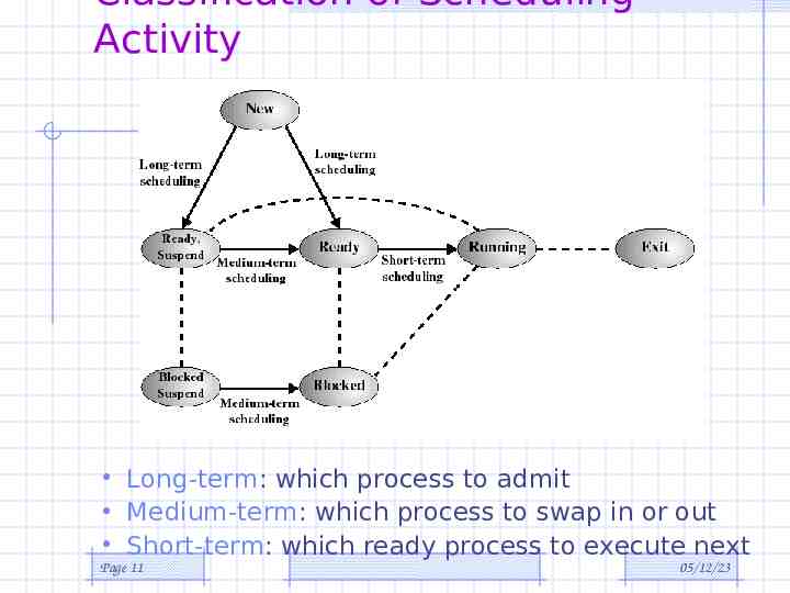
Classification of Scheduling Activity Long-term: which process to admit Medium-term: which process to swap in or out Short-term: which ready process to execute next Page 11 05/12/23
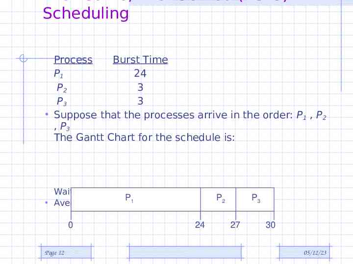
Scheduling Process Burst Time P1 24 P2 3 P3 3 Suppose that the processes arrive in the order: P1 , P2 , P3 The Gantt Chart for the schedule is: Waiting time for P1 0; P2 24; P3 27 P1 P P Average waiting time: (0 24 27)/32 17 3 0 Page 12 24 27 30 05/12/23
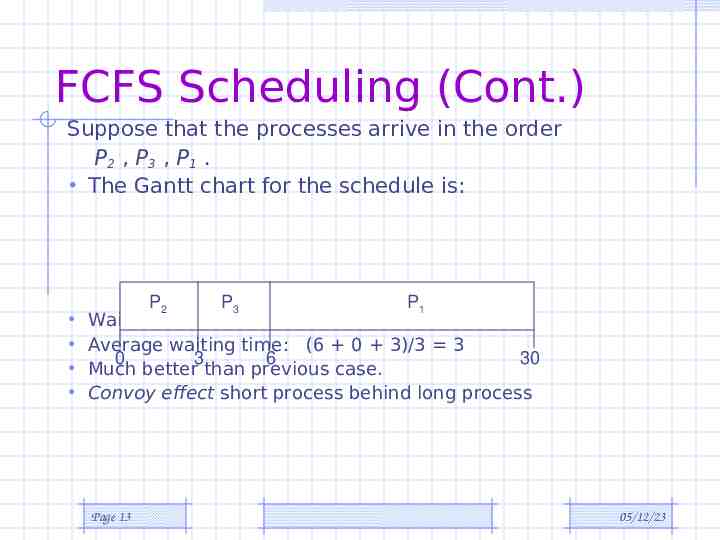
FCFS Scheduling (Cont.) Suppose that the processes arrive in the order P2 , P3 , P1 . The Gantt chart for the schedule is: P2 P3 P1 Waiting time for P1 6; P2 0; P3 3 Average waiting time: (6 0 3)/3 3 0 3 6 30 Much better than previous case. Convoy effect short process behind long process Page 13 05/12/23
Shortest-Job-First (SJR) Scheduling Associate with each process the length of its next CPU burst. Use these lengths to schedule the process with the shortest time. Two schemes: – nonpreemptive – once CPU given to the process it cannot be preempted until completes its CPU burst. – preemptive – if a new process arrives with CPU burst length less than remaining time of current executing process, preempt. This scheme is know as the Shortest-Remaining-Time-First (SRTF). SJF is optimal – gives minimum average waiting time for a given set of processes. Page 14 05/12/23
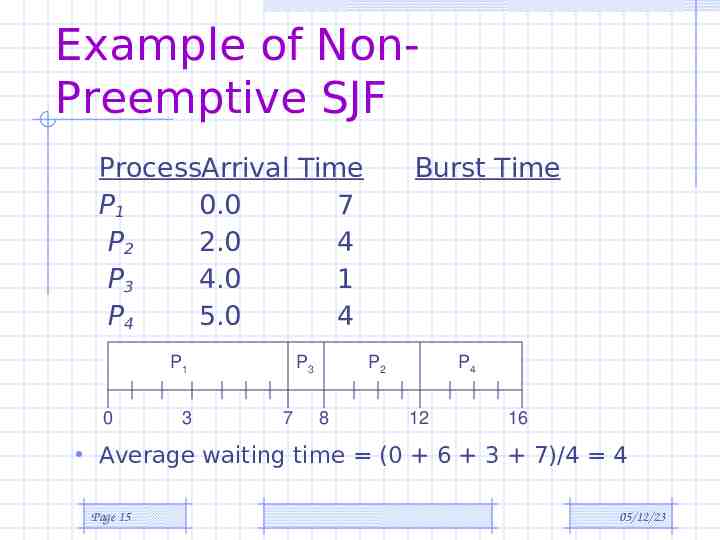
Example of NonPreemptive SJF ProcessArrival Time P1 0.0 7 P2 2.0 4 P3 4.0 1 P4 5.0 4 P1 0 3 P3 7 Burst Time P2 8 P4 12 16 Average waiting time (0 6 3 7)/4 4 Page 15 05/12/23
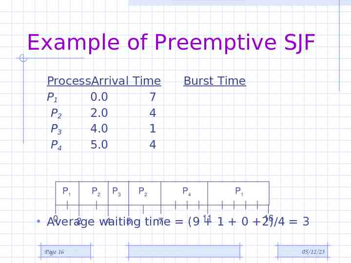
Example of Preemptive SJF ProcessArrival Time P1 0.0 7 P2 2.0 4 P3 4.0 1 P4 5.0 4 P1 P2 P3 P2 Burst Time P4 P1 16 0 2 4 5 7 (9 11 Average waiting time 1 0 2)/4 3 Page 16 05/12/23
Shortest job first: critique Possibility of starvation for longer processes as long as there is a steady supply of shorter processes Lack of preemption is not suited in a time sharing environment – CPU bound process gets lower priority (as it should) but a process doing no I/O could still monopolize the CPU if he is the first one to enter the system SJF implicitly incorporates priorities: shortest jobs are given preferences The next (preemptive) algorithm penalizes directly longer jobs Page 17 05/12/23
Priority Scheduling A priority number (integer) is associated with each process The CPU is allocated to the process with the highest priority (smallest integer highest priority). – Preemptive – nonpreemptive SJF is a priority scheduling where priority is the predicted next CPU burst time. Problem Starvation – low priority processes may never execute. Solution Aging – as time progresses increase the priority of the process. Page 18 05/12/23
Round Robin (RR) Each process gets a small unit of CPU time (time quantum), usually 10-100 milliseconds. After this time has elapsed, the process is preempted and added to the end of the ready queue. If there are n processes in the ready queue and the time quantum is q, then each process gets 1/n of the CPU time in chunks of at most q time units at once. No process waits more than (n-1)q time units. Performance – q large FIFO – q small q must be large with respect to context switch, otherwise overhead is too high. Page 19 05/12/23
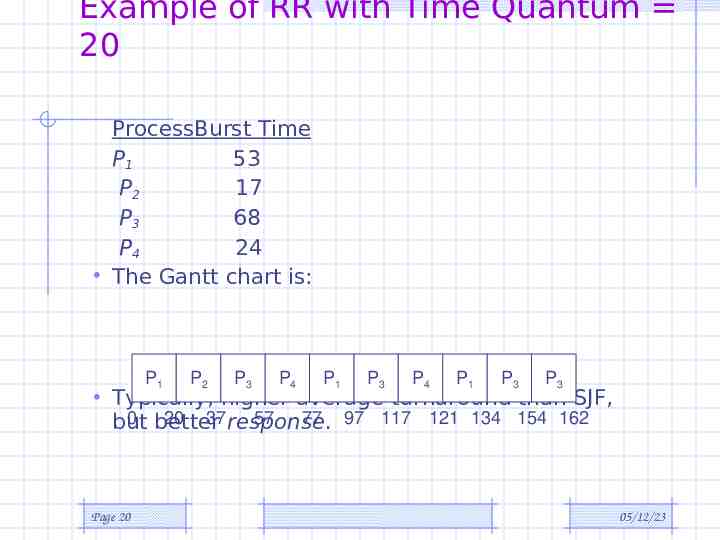
Example of RR with Time Quantum 20 ProcessBurst Time P1 53 P2 17 P3 68 P4 24 The Gantt chart is: P1 P2 P3 P4 P1 P3 P4 P1 P3 P3 Typically, higher average turnaround than SJF, 0 better 20 37 response. 57 77 97 117 121 134 154 162 but Page 20 05/12/23
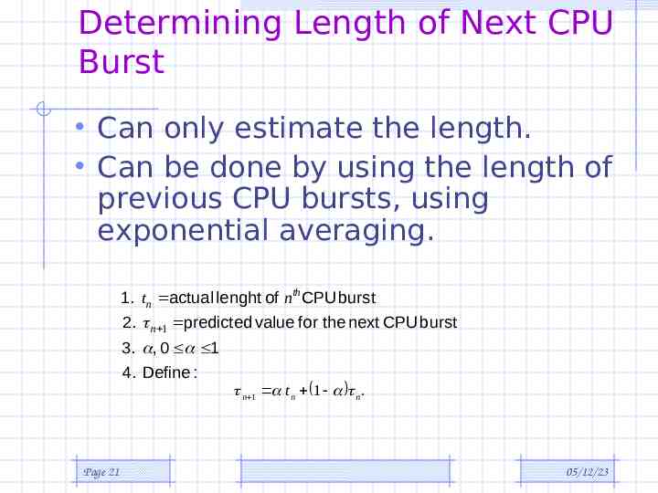
Determining Length of Next CPU Burst Can only estimate the length. Can be done by using the length of previous CPU bursts, using exponential averaging. 1. tn actual lenght of nthCPU burst 2. n 1 predicted value for the next CPU burst 3. , 0 1 4. Define : n 1 t n 1 n . Page 21 05/12/23
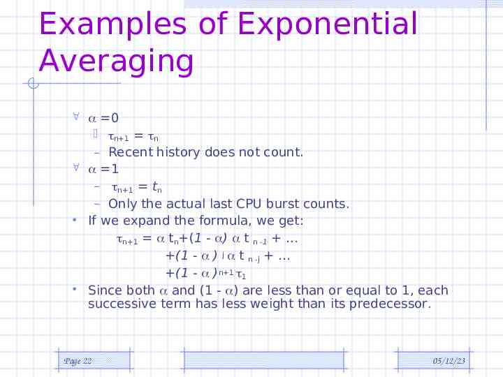
Examples of Exponential Averaging 0 n 1 n – Recent history does not count. 1 – n 1 tn – Only the actual last CPU burst counts. If we expand the formula, we get: n 1 tn (1 - ) t n -1 (1 - ) j t n -j (1 - )n 1 1 Since both and (1 - ) are less than or equal to 1, each successive term has less weight than its predecessor. Page 22 05/12/23
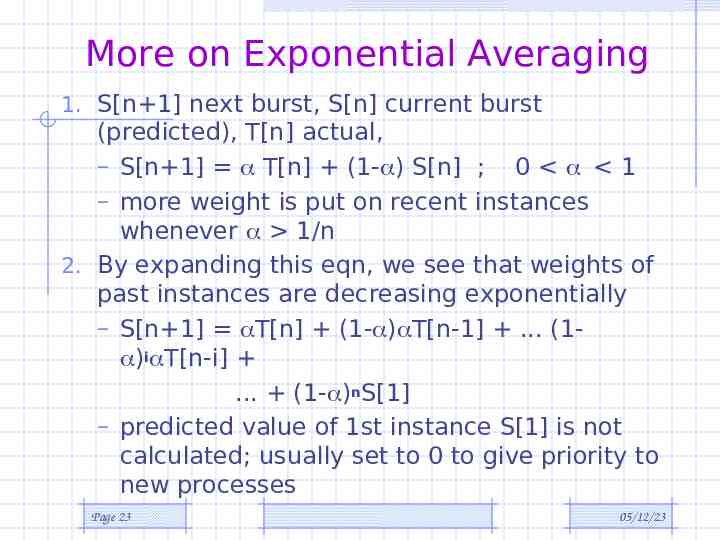
More on Exponential Averaging 1. S[n 1] next burst, S[n] current burst (predicted), T[n] actual, – S[n 1] T[n] (1- ) S[n] ; 0 1 – more weight is put on recent instances whenever 1/n 2. By expanding this eqn, we see that weights of past instances are decreasing exponentially – S[n 1] T[n] (1- ) T[n-1] . (1 )i T[n-i] . (1- )nS[1] – predicted value of 1st instance S[1] is not calculated; usually set to 0 to give priority to new processes Page 23 05/12/23
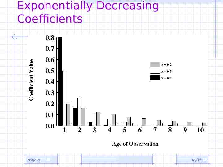
Exponentially Decreasing Coefficients Page 24 05/12/23
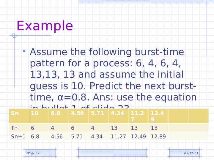
Example Assume the following burst-time Sn Tn pattern for a process: 6, 4, 6, 4, 13,13, 13 and assume the initial guess is 10. Predict the next bursttime, α 0.8. Ans: use the equation in bullet 1 of slide 23. 10 6.8 4.56 5.71 4.34 11.2 12.4 6 Sn 1 6.8 Page 25 7 9 13 13 4 6 4 13 4.56 5.71 4.34 11.27 12.49 12.89 05/12/23
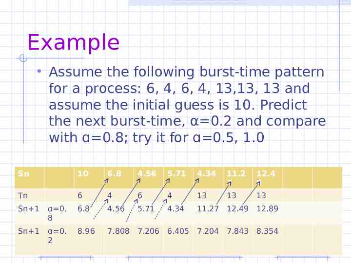
Example Assume the following burst-time pattern for a process: 6, 4, 6, 4, 13,13, 13 and assume the initial guess is 10. Predict the next burst-time, α 0.2 and compare with ɑ 0.8; try it for ɑ 0.5, 1.0 Sn 10 6.8 4.56 5.71 4.34 11.2 7 12.4 9 Tn 6 4 6 4 13 13 13 5.71 4.34 11.27 12.49 12.89 Sn 1 ɑ 0. 8 6.8 4.56 Sn 1 ɑ 0. 2 8.96 7.808 7.206 6.405 7.204 7.843 8.354 Page 26 05/12/23
Summary Scheduling is important for improving the system performance. Methods of prediction play an important role in Operating system and network functions. Simulation is a way of experimentally evaluating the performance of a technique. Next class we will examine queuing theory that allows for modeling of the scheduling disciplines. Page 27 05/12/23