Spatial Filtering CS474/674 – Prof. Bebis Sections 3.4, 3.5, 3.6,

58 Slides6.93 MB
Spatial Filtering CS474/674 - Prof. Bebis Sections 3.4, 3.5, 3.6, 3.7, 3.8
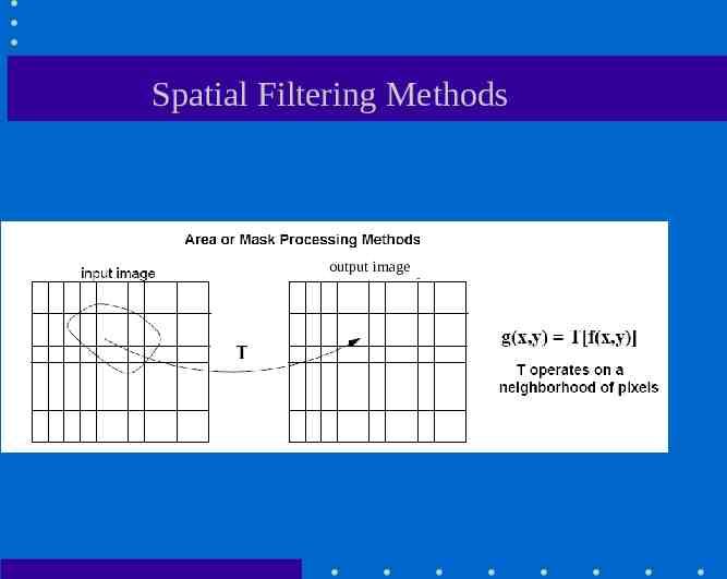
Spatial Filtering Methods output image
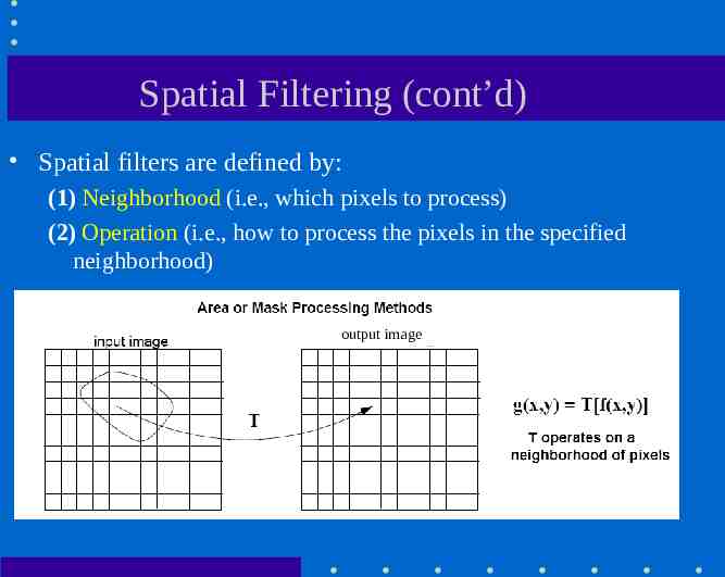
Spatial Filtering (cont’d) Spatial filters are defined by: (1) Neighborhood (i.e., which pixels to process) (2) Operation (i.e., how to process the pixels in the specified neighborhood) output image
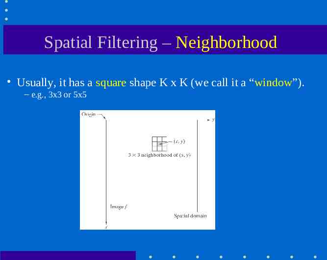
Spatial Filtering – Neighborhood Usually, it has a square shape K x K (we call it a “window”). – e.g., 3x3 or 5x5
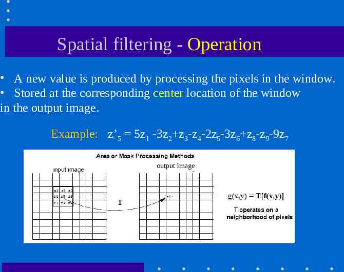
Spatial filtering - Operation A new value is produced by processing the pixels in the window. Stored at the corresponding center location of the window in the output image. Example: z’5 5z1 -3z2 z3-z4-2z5-3z6 z8-z9-9z7 output image
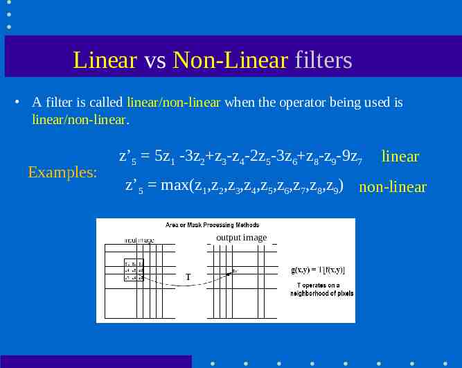
Linear vs Non-Linear filters A filter is called linear/non-linear when the operator being used is linear/non-linear. Examples: z’5 5z1 -3z2 z3-z4-2z5-3z6 z8-z9-9z7 linear z’5 max(z1,z2,z3,z4,z5,z6,z7,z8,z9) non-linear output image
Linear Operators Two common linear operators are: – Correlation – Convolution The output is a linear combination of the inputs.
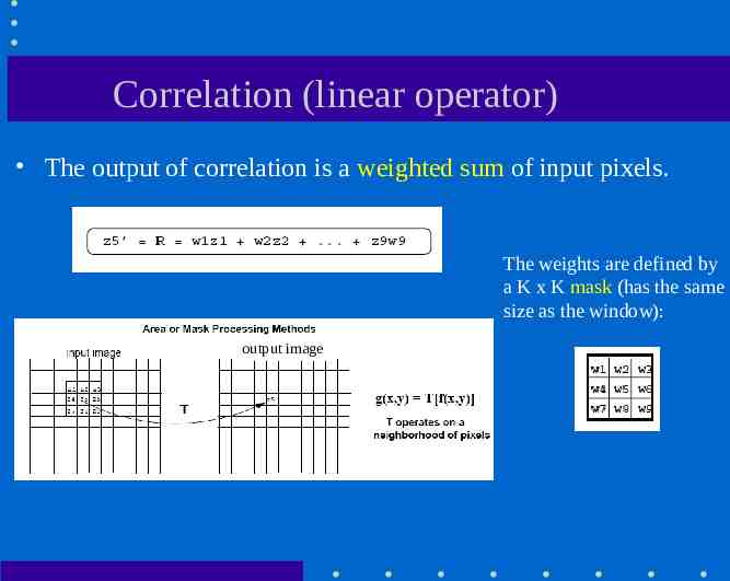
Correlation (linear operator) The output of correlation is a weighted sum of input pixels. The weights are defined by a K x K mask (has the same size as the window): output image
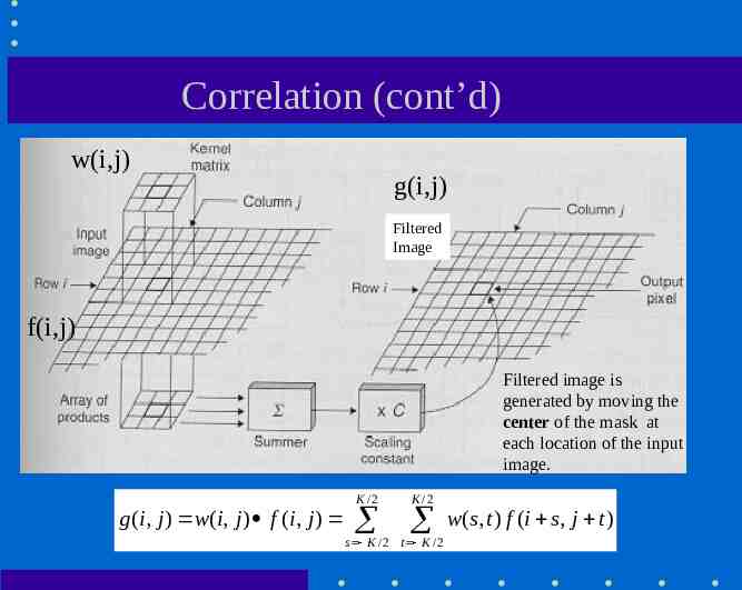
Correlation (cont’d) w(i,j) g(i,j) Filtered Image f(i,j) Filtered image is generated by moving the center of the mask at each location of the input image. g (i, j ) w(i, j ) f (i, j ) K /2 K /2 s K / 2 t K /2 w( s, t ) f (i s, j t )
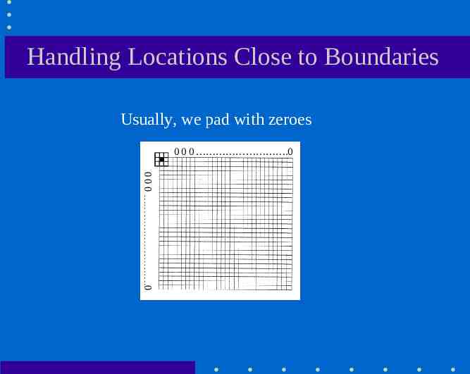
Handling Locations Close to Boundaries Usually, we pad with zeroes 0 0 0 .0 0 0 0 .0
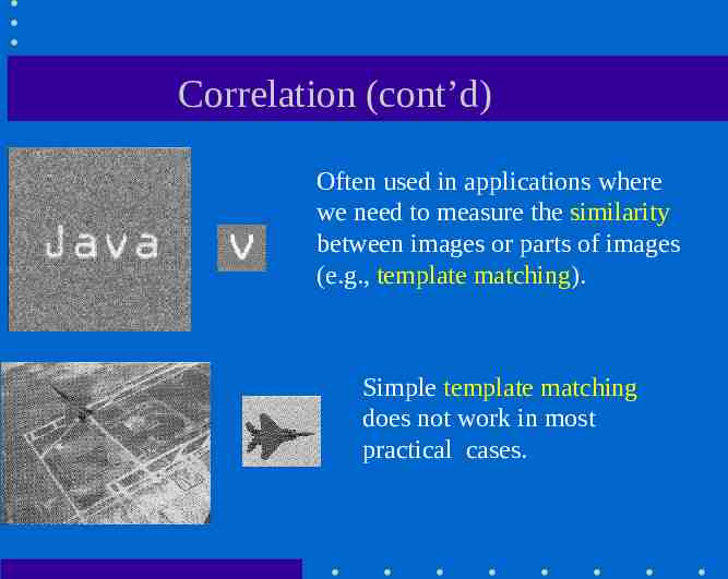
Correlation (cont’d) Often used in applications where we need to measure the similarity between images or parts of images (e.g., template matching). Simple template matching does not work in most practical cases.
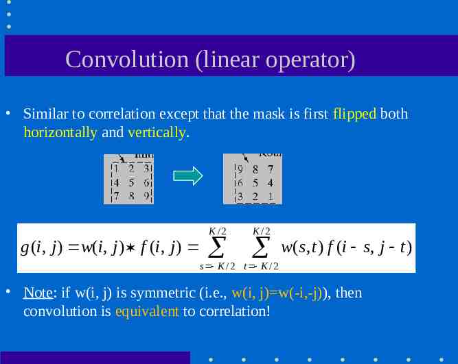
Convolution (linear operator) Similar to correlation except that the mask is first flipped both horizontally and vertically. g (i, j ) w(i, j ) f (i, j ) K /2 K /2 w( s, t ) f (i s, j t ) s K /2 t K /2 Note: if w(i, j) is symmetric (i.e., w(i, j) w(-i,-j)), then convolution is equivalent to correlation!
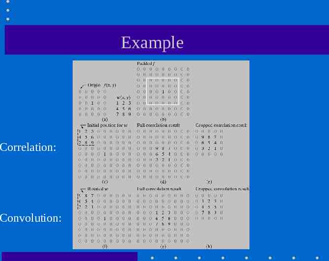
Example Correlation: Convolution:
Filter Categories We will focus on two types of filters: – Smoothing (also called “low-pass”) filters – Sharpening (also called “high-pass”) filters
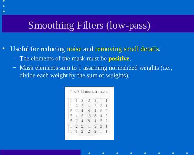
Smoothing Filters (low-pass) Useful for reducing noise and removing small details. – The elements of the mask must be positive. – Mask elements sum to 1 assuming normalized weights (i.e., divide each weight by the sum of weights).
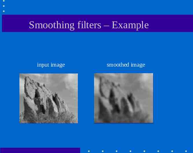
Smoothing filters – Example input image smoothed image
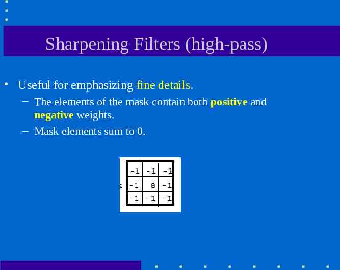
Sharpening Filters (high-pass) Useful for emphasizing fine details. – The elements of the mask contain both positive and negative weights. – Mask elements sum to 0.
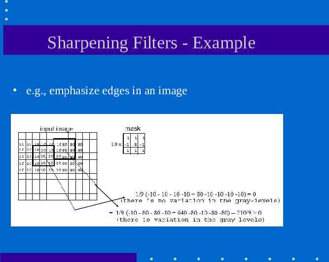
Sharpening Filters - Example e.g., emphasize edges in an image
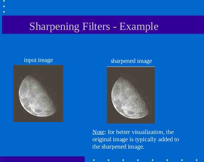
Sharpening Filters - Example input image sharpened image Note: for better visualization, the original image is typically added to the sharpened image.
Common Smoothing Filters Averaging (linear) Gaussian (linear) Median filtering (non-linear)
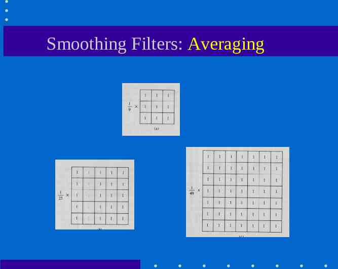
Smoothing Filters: Averaging
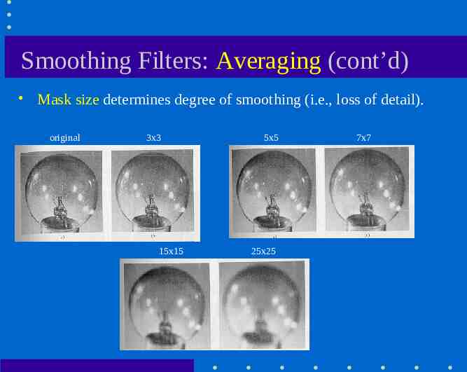
Smoothing Filters: Averaging (cont’d) Mask size determines degree of smoothing (i.e., loss of detail). original 3x3 15x15 5x5 25x25 7x7
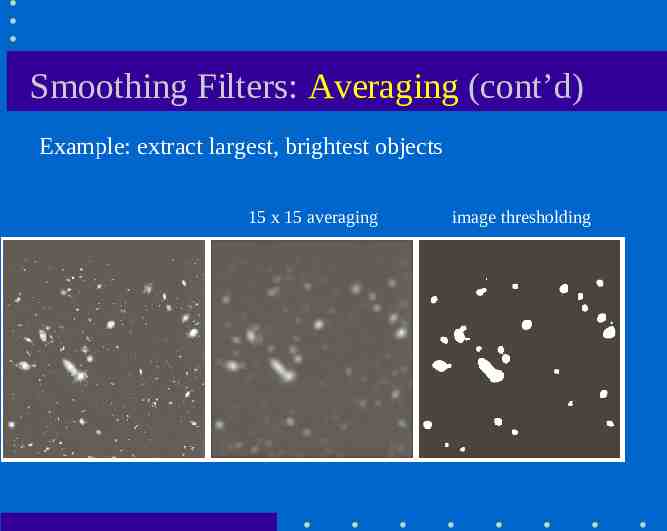
Smoothing Filters: Averaging (cont’d) Example: extract largest, brightest objects 15 x 15 averaging image thresholding
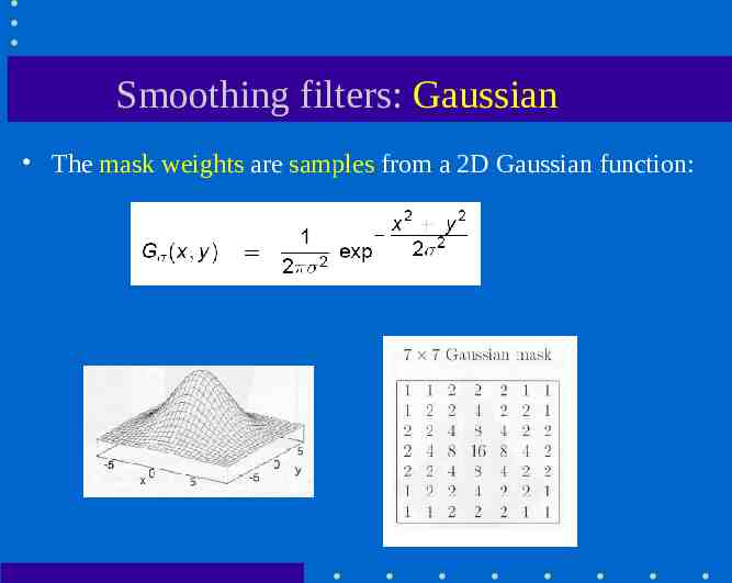
Smoothing filters: Gaussian The mask weights are samples from a 2D Gaussian function:
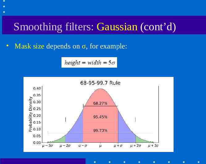
Smoothing filters: Gaussian (cont’d) Mask size depends on σ, for example:
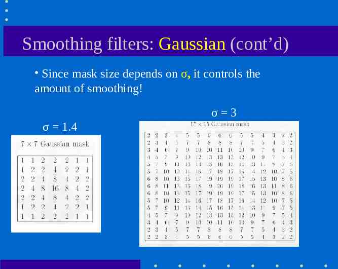
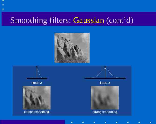
Smoothing filters: Gaussian (cont’d) Since mask size depends on σ, it controls the amount of smoothing! σ 3 σ 1.4
Smoothing filters: Gaussian (cont’d)
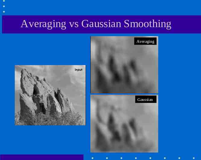
Averaging vs Gaussian Smoothing Averaging Gaussian
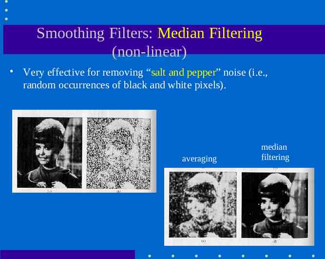
Smoothing Filters: Median Filtering (non-linear) Very effective for removing “salt and pepper” noise (i.e., random occurrences of black and white pixels). averaging median filtering
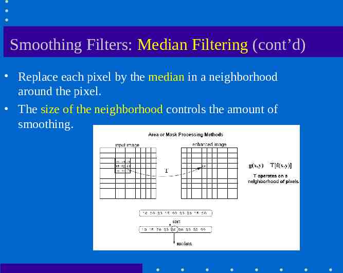
Smoothing Filters: Median Filtering (cont’d) Replace each pixel by the median in a neighborhood around the pixel. The size of the neighborhood controls the amount of smoothing.
Common Sharpening Filters Unsharp masking High Boost filtering Gradient (1st derivative) Laplacian (2nd derivative)
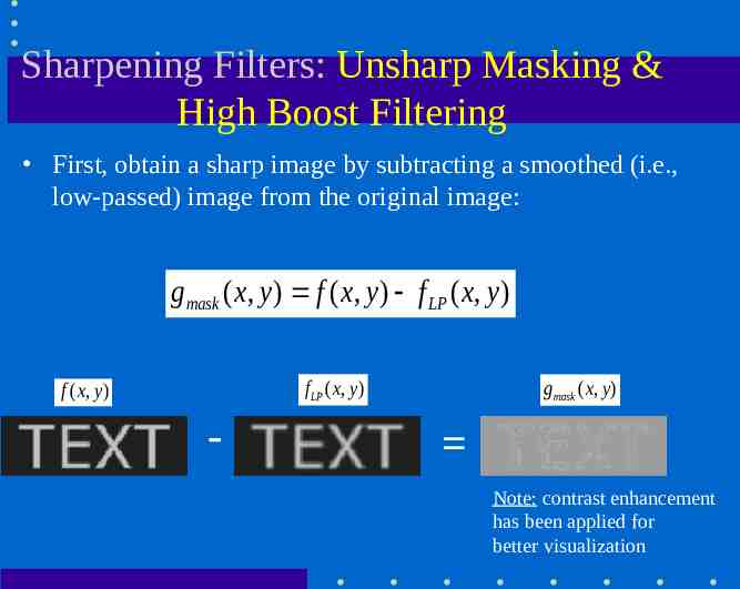
Sharpening Filters: Unsharp Masking & High Boost Filtering First, obtain a sharp image by subtracting a smoothed (i.e., low-passed) image from the original image: g mask ( x, y ) f ( x, y ) f LP ( x, y ) f LP ( x, y ) f ( x, y ) - g mask ( x, y ) Note: contrast enhancement has been applied for better visualization
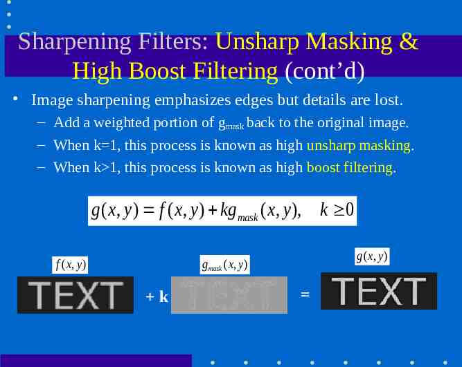
Sharpening Filters: Unsharp Masking & High Boost Filtering (cont’d) Image sharpening emphasizes edges but details are lost. – Add a weighted portion of gmask back to the original image. – When k 1, this process is known as high unsharp masking. – When k 1, this process is known as high boost filtering. g ( x, y ) f ( x, y ) kg mask ( x, y ), k 0 g ( x, y ) g mask ( x, y ) f ( x, y ) k
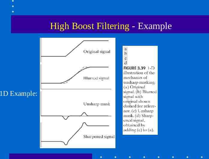
High Boost Filtering - Example 1D Example:
High Boost Filtering - Example original Gaussian smoothed 2D Example: gmask Unsharp Masking (k 1) Highboost Filtering (k 1)
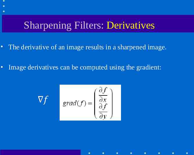
Sharpening Filters: Derivatives The derivative of an image results in a sharpened image. Image derivatives can be computed using the gradient:
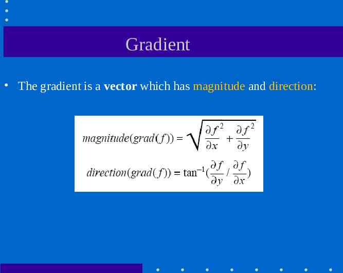
Gradient The gradient is a vector which has magnitude and direction:
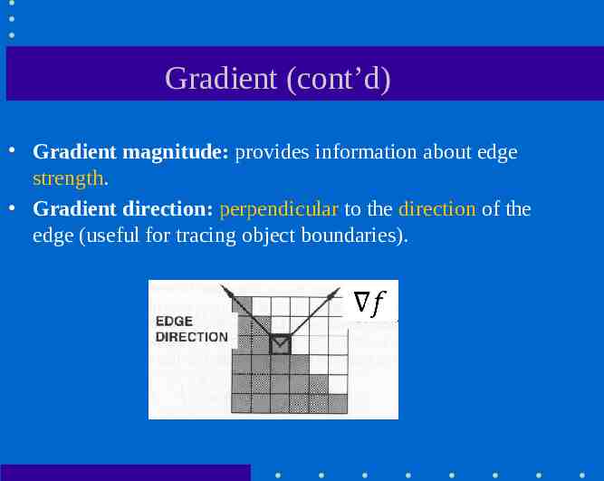
Gradient (cont’d) Gradient magnitude: provides information about edge strength. Gradient direction: perpendicular to the direction of the edge (useful for tracing object boundaries).
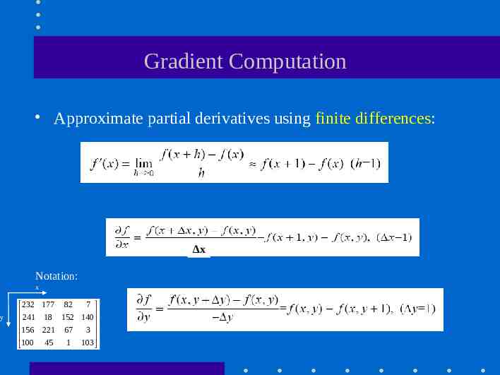
Gradient Computation Approximate partial derivatives using finite differences: Δx Notation: x y 7 232 177 82 241 18 152 140 156 221 67 3 1 103 100 45
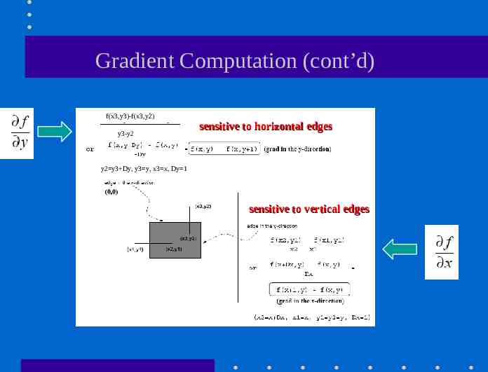
Gradient Computation (cont’d) f(x3,y3)-f(x3,y2) y3-y2 sensitive to horizontal edges y2 y3 Dy, y3 y, x3 x, Dy 1 sensitive to vertical edges
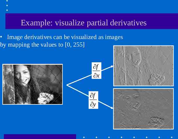
Example: visualize partial derivatives Image derivatives can be visualized as images by mapping the values to [0, 255] f x f y
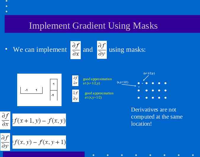
Implement Gradient Using Masks We can implement and using masks: (x 1/2,y) good approximation at (x 1/2,y) (x,y 1/2) * * good approximation at (x,y 1/2) Derivatives are not computed at the same location!
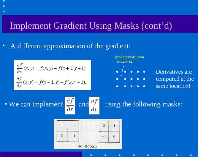
Implement Gradient Using Masks (cont’d) A different approximation of the gradient: good approximation (x 1/2,y 1/2) * We can implement and Derivatives are computed at the same location! using the following masks:
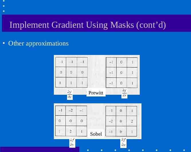
Implement Gradient Using Masks (cont’d) Other approximations Prewitt Sobel
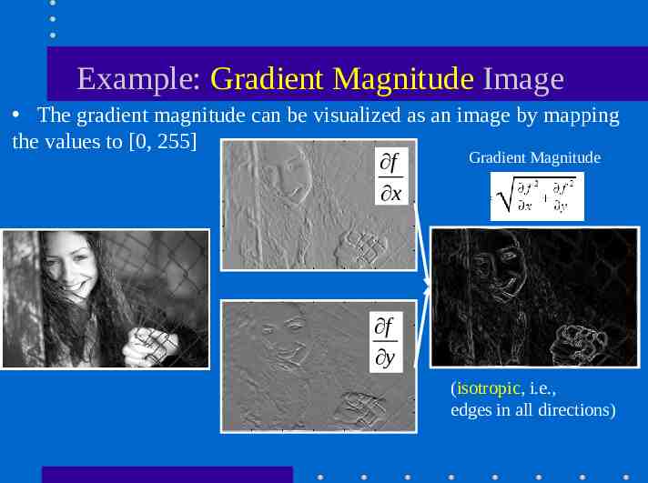
Example: Gradient Magnitude Image The gradient magnitude can be visualized as an image by mapping the values to [0, 255] Gradient Magnitude f x f y (isotropic, i.e., edges in all directions)
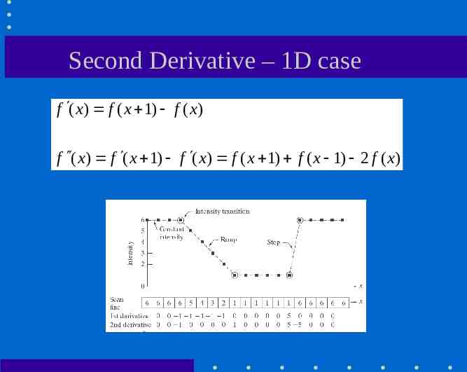
Second Derivative – 1D case f ( x) f ( x 1) f ( x) f ( x) f ( x 1) f ( x) f ( x 1) f ( x 1) 2 f ( x)
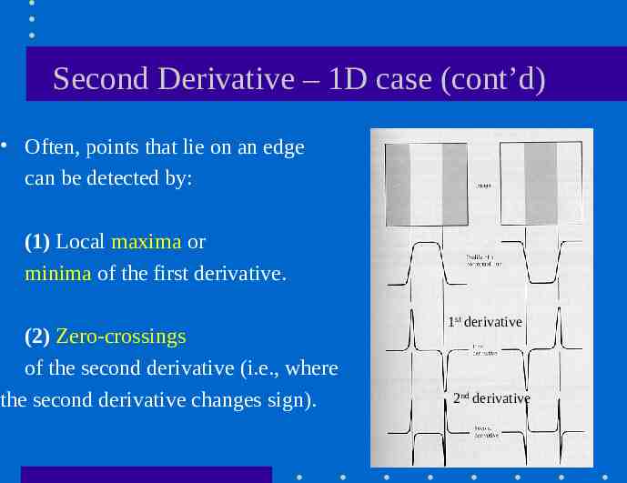
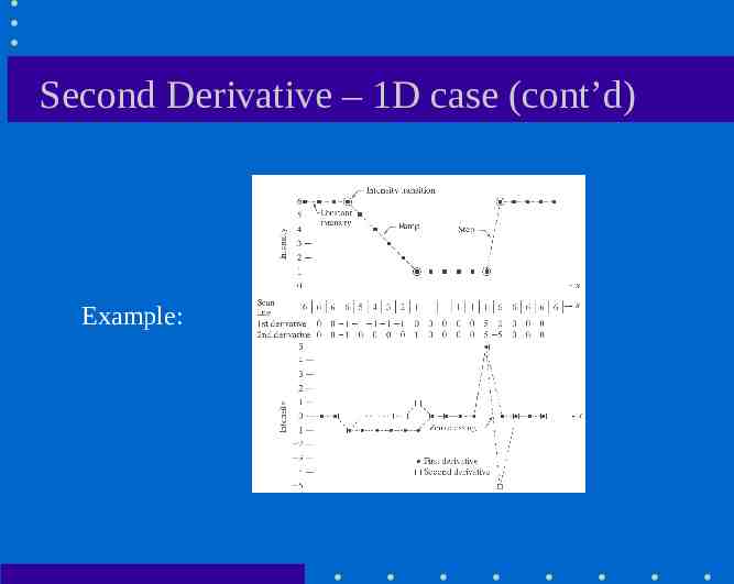
Second Derivative – 1D case (cont’d) Often, points that lie on an edge can be detected by: (1) Local maxima or minima of the first derivative. (2) Zero-crossings of the second derivative (i.e., where the second derivative changes sign). 1st derivative 2nd derivative
Second Derivative – 1D case (cont’d) Example:
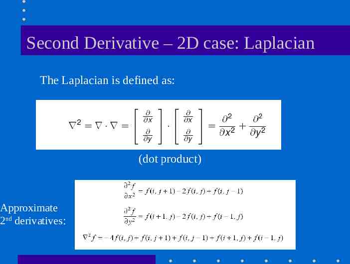
Second Derivative – 2D case: Laplacian The Laplacian is defined as: (dot product) Approximate 2nd derivatives:
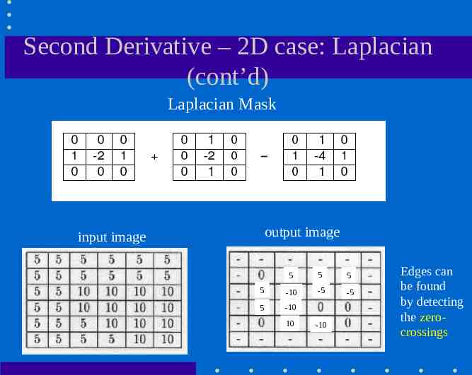
Second Derivative – 2D case: Laplacian (cont’d) Laplacian Mask output image input image 5 5 5 5 -10 -5 -5 5 -10 10 -10 Edges can be found by detecting the zerocrossings
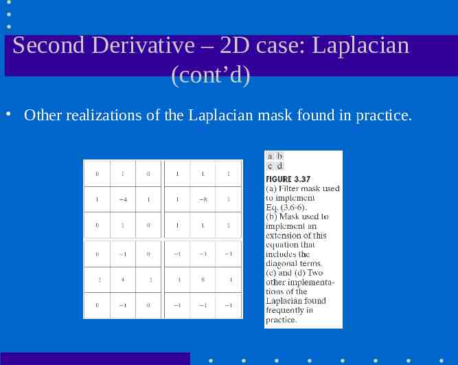
Second Derivative – 2D case: Laplacian (cont’d) Other realizations of the Laplacian mask found in practice.
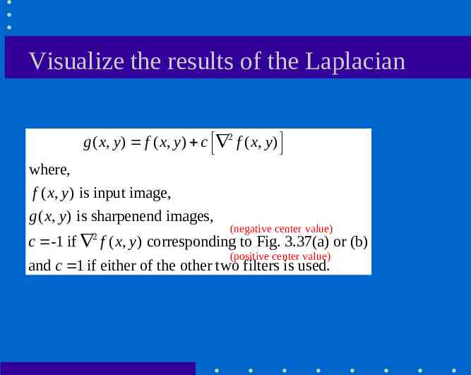
Visualize the results of the Laplacian g ( x, y ) f ( x, y ) c 2 f ( x, y ) where, f ( x, y ) is input image, g ( x, y ) is sharpenend images, 2 (negative center value) c -1 if f ( x, y ) corresponding to Fig. 3.37(a) or (b) (positive center value) and c 1 if either of the other two filters is used.
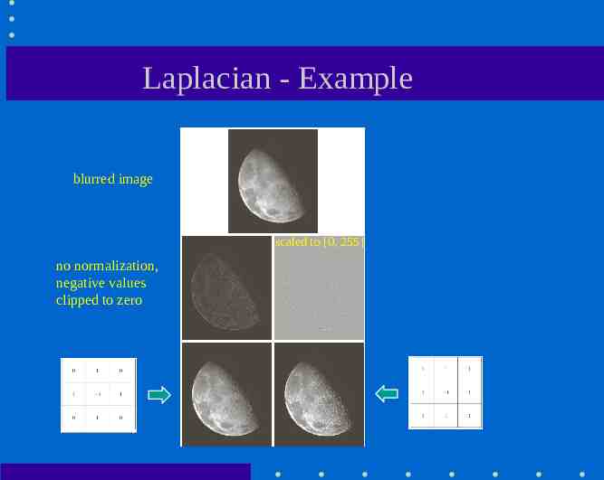
Laplacian - Example blurred image scaled to [0, 255] no normalization, negative values clipped to zero
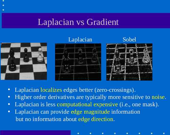
Laplacian vs Gradient Laplacian Sobel Laplacian localizes edges better (zero-crossings). Higher order derivatives are typically more sensitive to noise. Laplacian is less computational expensive (i.e., one mask). Laplacian can provide edge magnitude information but no information about edge direction.
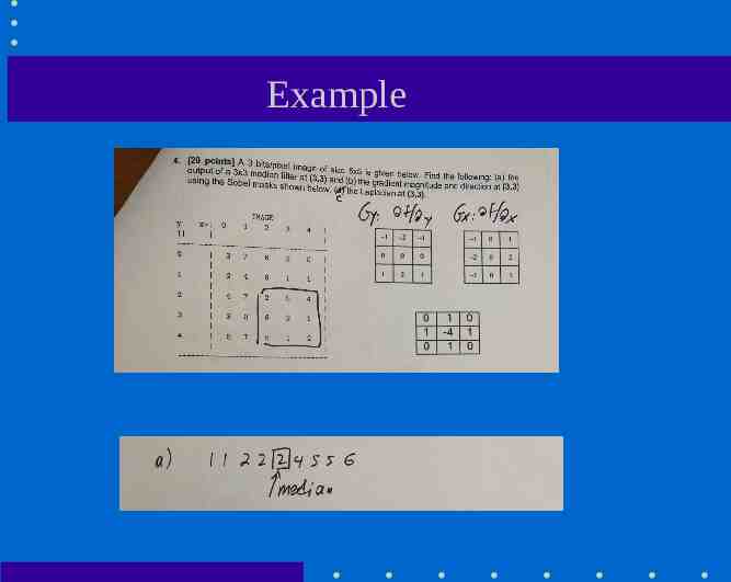
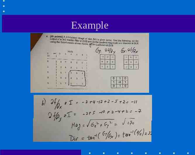
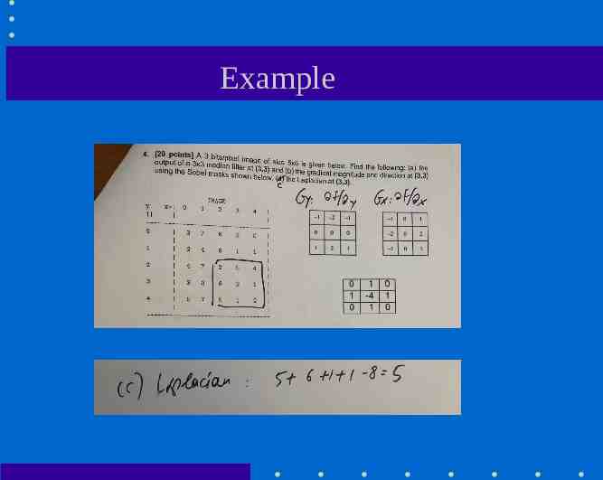
Example
Example
Example
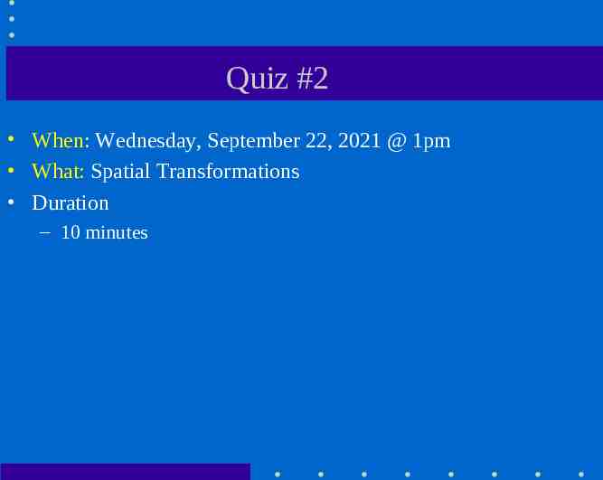
Quiz #2 When: Wednesday, September 22, 2021 @ 1pm What: Spatial Transformations Duration – 10 minutes