Review for Final Exam Some important themes from Chapters 9-11 Final

19 Slides88.00 KB
Review for Final Exam Some important themes from Chapters 9-11 Final exam covers these chapters, but implicitly tests the entire course, because we use sampling distributions, confidence intervals, significance tests, etc. As usual, exam is mixture of true/false to test concepts and problems (like examples in class and homework), with emphasis on interpreting software output.
Chap. 9: Linear Regression and Correlation Data: y – a quantitative response variable x – a quantitative explanatory variable We consider: Is there an association? (test of independence using slope) How strong is the association? (uses correlation r and r2) How can we predict y using x? (estimate a regression equation) Linear regression equation E(y) x describes how mean of conditional distribution of y changes as x changes Least squares estimates this and provides a sample prediction equation yˆ a bx
The linear regression equation E(y) x is part of a model. The model has another parameter σ that describes the variability of the conditional distributions; that is, the variability of y values for all subjects having the same x-value. For an observation, difference y yˆ between observed value of y and predicted value ŷ of y, is a residual (vertical distance on scatterplot) Least squares method minimizes the sum of squared residuals (errors), which is SSE used also in r2 and the estimate s of conditional standard deviation of y
Measuring association: The correlation and its square The correlation is a standardized slope that does not depend on units Correlation r relates to slope b of prediction equation by r b(sx/sy) -1 r 1, with r having same sign as b and r 1 or -1 when all sample points fall exactly on prediction line, so r describes strength of linear association The larger the absolute value, the stronger the association Correlation implies that predictions regress toward the mean
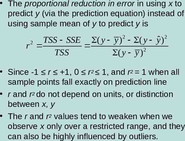
The proportional reduction in error in using x to predict y (via the prediction equation) instead of using sample mean of y to predict y is 2 2 ˆ TSS SSE ( y y ) ( y y ) r2 TSS ( y y ) 2 Since -1 r 1, 0 r2 1, and r2 1 when all sample points fall exactly on prediction line r and r2 do not depend on units, or distinction between x, y The r and r2 values tend to weaken when we observe x only over a restricted range, and they can also be highly influenced by outliers.
Inference for regression model Parameter: Population slope in regression model ( ) H0: independence is H0: 0 Test statistic t (b – 0)/se, with df n – 2 A CI for has form b t(se) where t-score has df n-2 and is from t-table with half the error probability in each tail. (Same se as in test) In practice, CI for multiple of slope (e.g., 10 ) may be more relevant (find by multiplying endpoints of CI for by the relevant constant) CI not containing 0 is equivalent to rejecting H 0 (when error probability is same for each)
Software reports SS values (SSE, regression SS, TSS regression SS SSE) and F test results in an ANOVA (analysis of variance) table The F statistic in the ANOVA table is the square of the t statistic for testing H0: 0. It has the same P-value as for the two-sided test. We need to use F when we have several parameters in H0 , such as in testing that all parameters in a multiple regression model 0 (see Chapter 11)
Chap. 10: Introduction to Multivariate Relationships Bivariate analyses informative, but we usually need to take into account many variables. Many explanatory variables have an influence on any particular response variable. The effect of an explanatory variable on a response variable may change when we take into account other variables. (Recall admissions into Berkeley example) When each pair of variables is associated, then a bivariate association for two variables may differ from its “partial” association, controlling for another variable
Association does not imply causation! With observational data, effect of X on Y may be partly due to association of X and Y with other lurking variables. Experimental studies have advantage of being able to control potential lurking variables (groups being compared should be roughly “balanced” on them). When X1 and X2 both have effects on Y but are also associated with each other, there is confounding. It’s difficult to determine whether either truly causes Y, because a variable’s effect could be at least partially due to its association with the other variable.
Simpson’s paradox: It is possible for the (bivariate) association between two variables to be positive, yet for the partial association to be negative at each fixed level of a third variable (or reverse) Spurious association: Y and X1 both depend on X2 and association disappears after controlling X2 Multiple causes more common, in which explanatory variables have associations among themselves as well as with response var. Effect of any one changes depending on what other variables controlled (statistically), often because it has a direct effect and also indirect effects. Statistical interaction – Effect of X1 on Y changes as the level of X2 changes (e.g., non-parallel lines in regr.)
Chap. 11: Multiple Regression y – response variable x1, x2 , , xk -- set of explanatory variables All variables assumed to be quantitative (later chapters incorporate categorical variables in model also) Multiple regression equation (population): E(y) 1x1 2x2 . kxk Controlling for other predictors in model, there is a linear relationship between E(y) and x1 with slope 1.
Partial effects in multiple regression refer to statistically controlling other variables in model, so differ from effects in bivariate models, which ignore all other variables. Partial effect of a predictor in multiple regression is identical at all fixed values of other predictors in model (assumption of “no interaction,” corresponding to parallel lines) Again, this is a model. We fit it using least squares, minimizing SSE out of all equations of the assumed form. The model may not be appropriate (e.g., if there is severe interaction). Graphics include scatterplot matrix (corresponding to correlation matrix), partial regression plots to study effect of a predictor after controlling (instead of ignoring) other var’s.
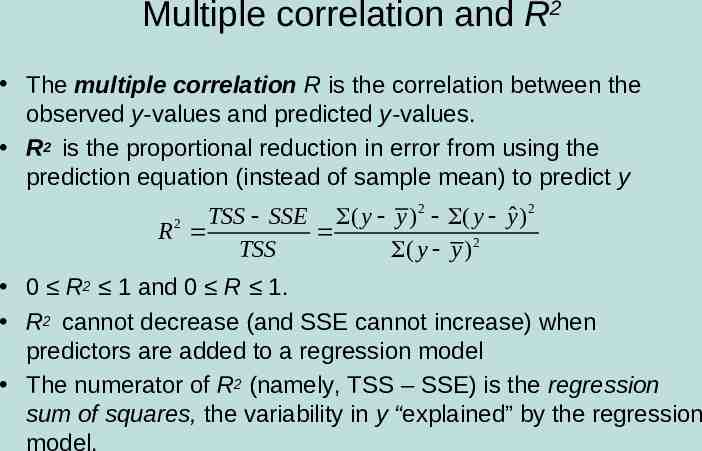
Multiple correlation and R2 The multiple correlation R is the correlation between the observed y-values and predicted y-values. R2 is the proportional reduction in error from using the prediction equation (instead of sample mean) to predict y TSS SSE ( y y ) 2 ( y yˆ ) 2 R TSS ( y y ) 2 2 0 R2 1 and 0 R 1. R2 cannot decrease (and SSE cannot increase) when predictors are added to a regression model The numerator of R2 (namely, TSS – SSE) is the regression sum of squares, the variability in y “explained” by the regression model.
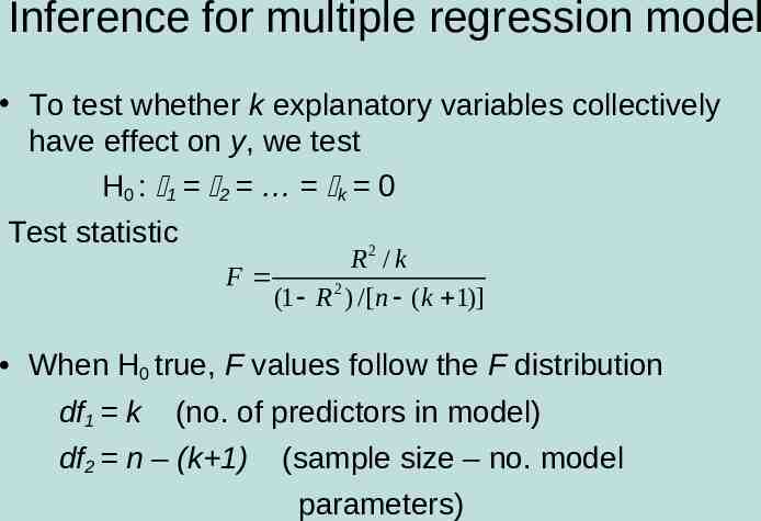
Inference for multiple regression model To test whether k explanatory variables collectively have effect on y, we test H0 : 1 2 k 0 Test statistic R2 / k F (1 R 2 ) /[n (k 1)] When H0 true, F values follow the F distribution df1 k (no. of predictors in model) df2 n – (k 1) (sample size – no. model parameters)
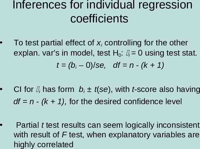
Inferences for individual regression coefficients To test partial effect of xi controlling for the other explan. var’s in model, test H0: i 0 using test stat. t (bi – 0)/se, df n - (k 1) CI for i has form bi t(se), with t-score also having df n - (k 1), for the desired confidence level Partial t test results can seem logically inconsistent with result of F test, when explanatory variables are highly correlated
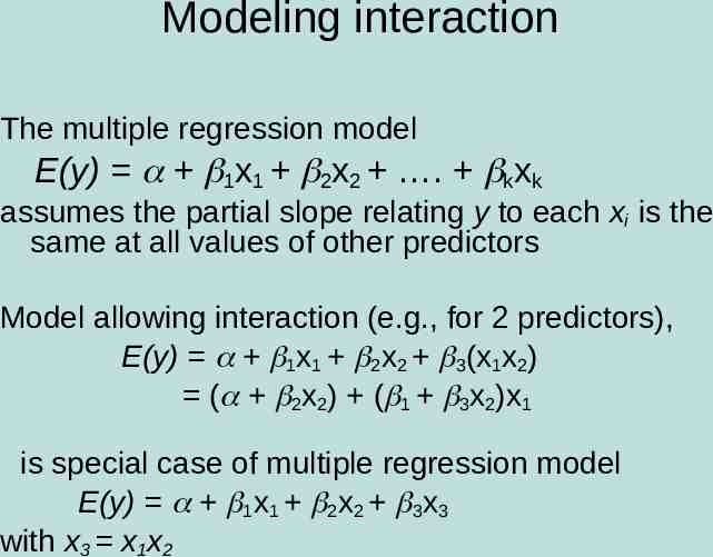
Modeling interaction The multiple regression model E(y) 1x1 2x2 . kxk assumes the partial slope relating y to each xi is the same at all values of other predictors Model allowing interaction (e.g., for 2 predictors), E(y) 1x1 2x2 3(x1x2) ( 2x2) ( 1 3x2)x1 is special case of multiple regression model E(y) 1x1 2x2 3x3 with x3 x1x2
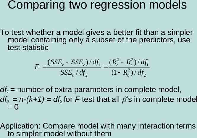
Comparing two regression models To test whether a model gives a better fit than a simpler model containing only a subset of the predictors, use test statistic ( SSEr SSEc ) / df1 ( Rc2 Rr2 ) / df1 F SSEc / df 2 (1 Rc2 ) / df 2 df1 number of extra parameters in complete model, df2 n-(k 1) df2 for F test that all ’s in complete model 0 Application: Compare model with many interaction terms to simpler model without them
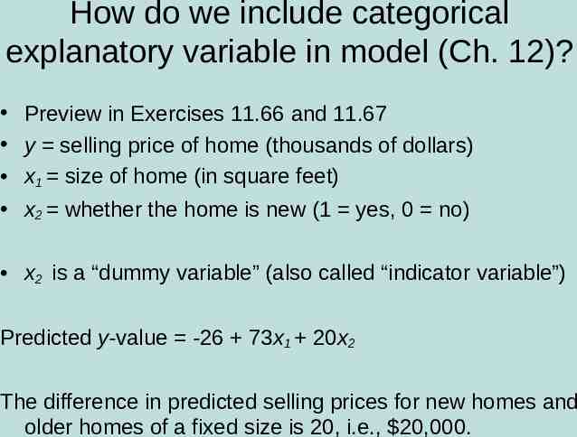
How do we include categorical explanatory variable in model (Ch. 12)? Preview in Exercises 11.66 and 11.67 y selling price of home (thousands of dollars) x1 size of home (in square feet) x2 whether the home is new (1 yes, 0 no) x2 is a “dummy variable” (also called “indicator variable”) Predicted y-value -26 73x1 20x2 The difference in predicted selling prices for new homes and older homes of a fixed size is 20, i.e., 20,000.
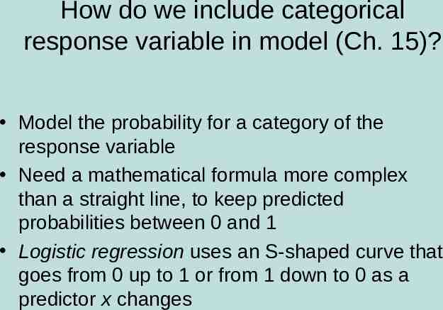
How do we include categorical response variable in model (Ch. 15)? Model the probability for a category of the response variable Need a mathematical formula more complex than a straight line, to keep predicted probabilities between 0 and 1 Logistic regression uses an S-shaped curve that goes from 0 up to 1 or from 1 down to 0 as a predictor x changes