Ordinary least Squares

21 Slides56.00 KB
Ordinary least Squares
Introduction Describe the nature of financial data. Assess the concepts underlying regressions analysis Describe some examples of financial models. Examine the Ordinary least Squares (OLS) technique and hypothesis testing
Financial data The data can be high frequency, i.e. daily or even every minute. i.e. Stock market prices are measured every time there is a trade or somebody posts a new quote. The data is usually good quality Recorded asset prices are usually those at which the transaction took place. Little possibility for measurement error.
Financial Data Financial Data is affected by risk. Most financial data is affected by not just return but also risk, which requires specialist modelling. Financial data is ‘noisy’ It is often difficult to pick up patterns in the data due to the variable nature of financial data.
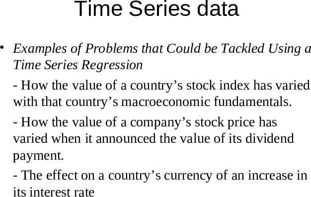
Time Series data Examples of Problems that Could be Tackled Using a Time Series Regression - How the value of a country’s stock index has varied with that country’s macroeconomic fundamentals. - How the value of a company’s stock price has varied when it announced the value of its dividend payment. - The effect on a country’s currency of an increase in its interest rate
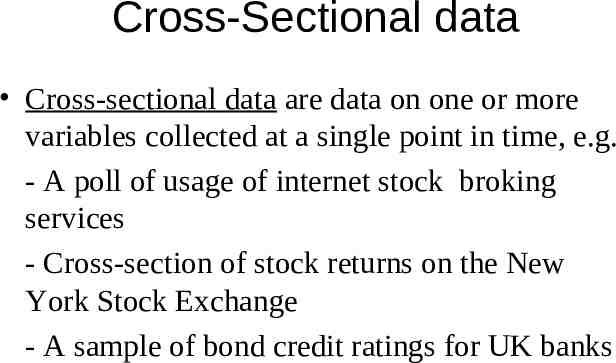
Cross-Sectional data Cross-sectional data are data on one or more variables collected at a single point in time, e.g. - A poll of usage of internet stock broking services - Cross-section of stock returns on the New York Stock Exchange - A sample of bond credit ratings for UK banks
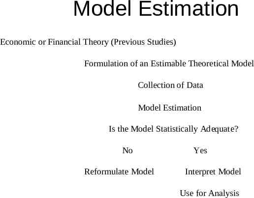
Model Estimation Economic or Financial Theory (Previous Studies) Formulation of an Estimable Theoretical Model Collection of Data Model Estimation Is the Model Statistically Adequate? No Reformulate Model Yes Interpret Model Use for Analysis
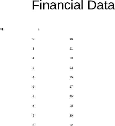
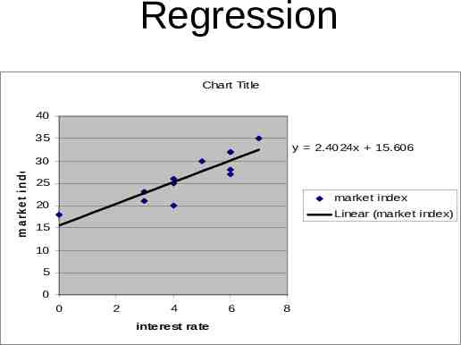
Financial Data MI i 0 18 3 21 4 20 3 23 4 25 6 27 4 26 6 28 5 30 6 32
Regression Chart Title 40 m a rk et in d e x 35 y 2.4024x 15.606 30 25 market index 20 Linear (market index) 15 10 5 0 0 2 4 interest rate 6 8
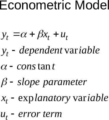
Econometric Model yt xt ut yt dependent var iable cons tan t slope parameter xt exp lanatory var iable ut error term
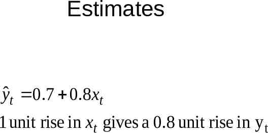
Estimates yˆ t 0.7 0.8 xt 1 unit rise in xt gives a 0.8 unit rise in y t
The Residual Term (Also called the error term and disturbance term) It describes the random component of the regression. It is caused by: - Omission of explanatory variables - The aggregation of the variables - Mis-specification of the model - Incorrect functional form of the model - Measurement error
Least Squares Approach The aim of this approach is to minimize the residual for all residuals We square the residual before minimizing We can then derive our intercept and slope parameter using basic calculus
Regression Regression is the degree of dependency of the dependent variable on the explanatory variables Correlation measures the strength of a linear association between two variables Causation suggests the dependent variable depends on previous values of the explanatory variable Regression does not imply causaltion
R-Squared Statistic This statistic explains the proportion of total variation in the dependent variable which is explained by the regression The statistic explains the explanatory power of the regression and measures how good a fit the data is. The value of this statistic lies between 0 and 1(when all the scatter plots lie on the regression line.)
Interpretation of Results Consider the type of model being estimated What are the units of measurement of the variables (unless all the variables are in logarithmic form) The range of observations The signs of the variables, does it accord with the theoretical model Are the magnitudes of the parameters plausible We need to remember it is only a model, the parameters are estimates, so it describes average values, individual cases may vary
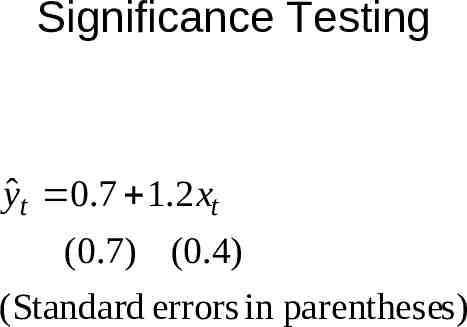
Significance Testing yˆ t 0.7 1.2 xt (0.7) (0.4) (Standard errors in parentheses)
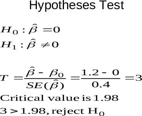
Hypotheses Test H 0 : ˆ 0 H : ˆ 0 1 ˆ 0 1.2 0 T 3 0.4 SE ( ˆ ) Critical value is 1.98 3 1.98, reject H 0
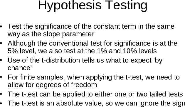
Hypothesis Testing Test the significance of the constant term in the same way as the slope parameter Although the conventional test for significance is at the 5% level, we also test at the 1% and 10% levels Use of the t-distribution tells us what to expect ‘by chance’ For finite samples, when applying the t-test, we need to allow for degrees of freedom The t-test can be applied to either one or two tailed tests The t-test is an absolute value, so we can ignore the sign
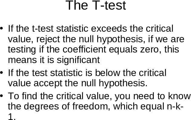
The T-test If the t-test statistic exceeds the critical value, reject the null hypothesis, if we are testing if the coefficient equals zero, this means it is significant If the test statistic is below the critical value accept the null hypothesis. To find the critical value, you need to know the degrees of freedom, which equal n-k1.
Conclusion Financial data tends to be more plentiful and of better quality than other data. Regression analysis involves fitting a line to a scatter diagram The error term describes the random component of the regression Ordinary Least Squares (OLS) involves minimizing the sum of the square of the residuals