Neural Network Architectures Geoff Hulten


22 Slides2.54 MB
Neural Network Architectures Geoff Hulten
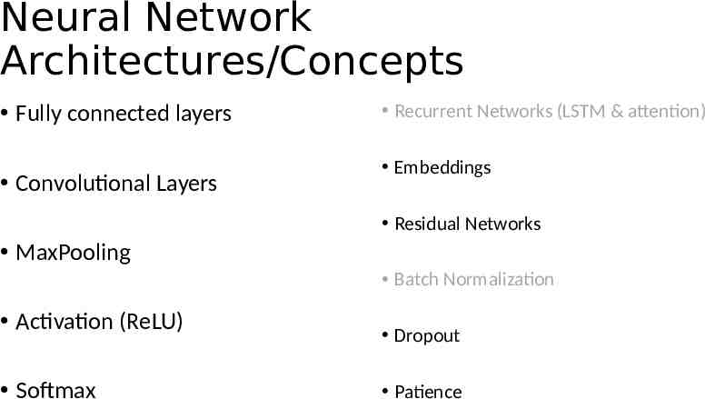
Neural Network Architectures/Concepts Fully connected layers Convolutional Layers Recurrent Networks (LSTM & attention) Embeddings Residual Networks MaxPooling Batch Normalization Activation (ReLU) Softmax Dropout Patience
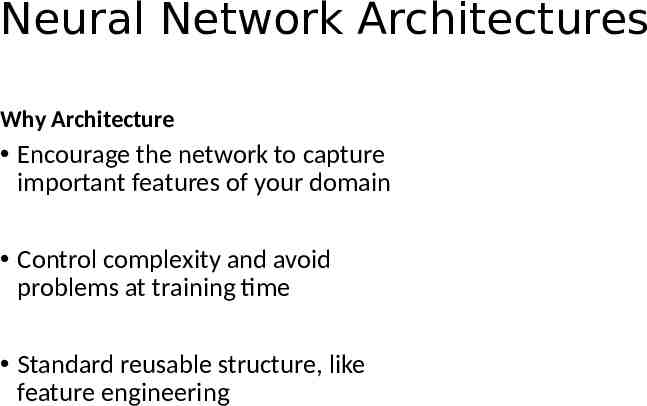
Neural Network Architectures Why Architecture Encourage the network to capture important features of your domain Control complexity and avoid problems at training time Standard reusable structure, like feature engineering
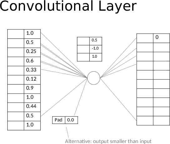
Convolutional Layer 1.0 0.5 0.5 0.25 0.6 -1.0 0.25 1.0 0.85 0.23 0.33 0.29 0.12 1.28 0.9 0.6 1.0 -0.06 0.44 0.5 1.0 0 0.56 Pad 0.0 Alternative: output smaller than input 0.0
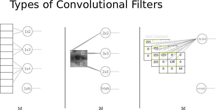
Types of Convolutional Filters 1x2 1x3 2x2 3x3 Red Channel 255 Green 255 255 Channel 0 255 0 Channel 0 0 Blue 255 0 255 00 0 255 255 1x4 1xN 1d 2x3 2x2x3 00 0 0 128 255 0 0 0 64 0 MxN 2d MxNxD 3d
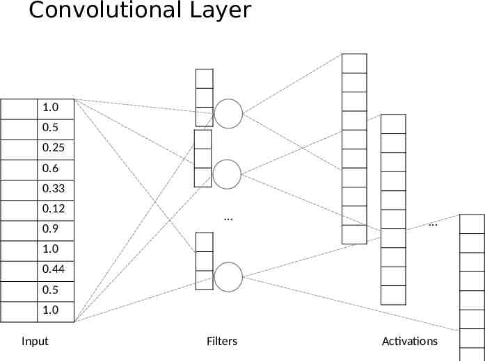
Convolutional Layer 1.0 0.5 0.25 0.6 0.33 0.12 0.9 1.0 0.44 0.5 1.0 Input Filters Activations
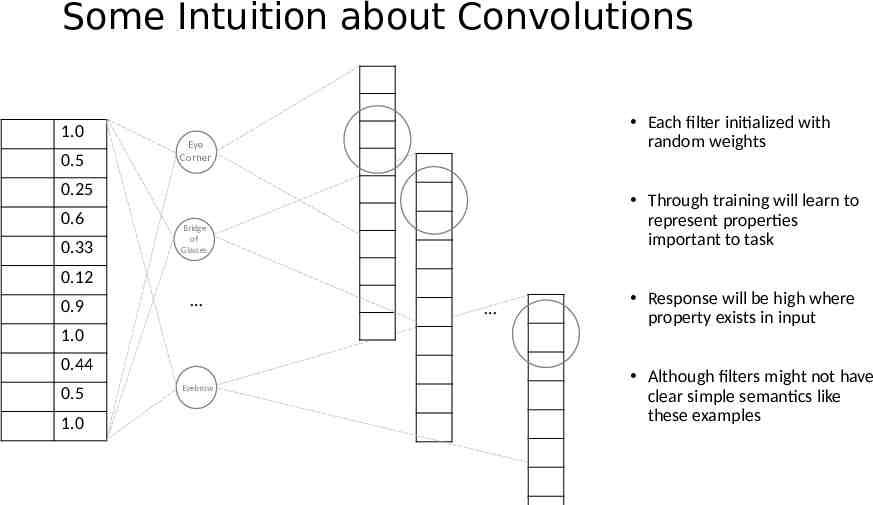
Some Intuition about Convolutions 1.0 0.5 Each filter initialized with random weights Eye Corner 0.25 0.6 0.33 Through training will learn to represent properties important to task Bridge of Glasses 0.12 0.9 1.0 0.44 0.5 1.0 Eyebrow Response will be high where property exists in input Although filters might not have clear simple semantics like these examples
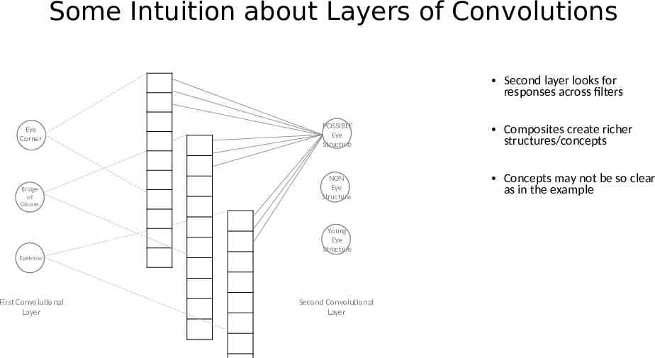
Some Intuition about Layers of Convolutions Second layer looks for responses across filters Eye Corner Bridge of Glasses POSSIBLE Eye Structure NON Eye Structure Young Eye Structure Eyebrow First Convolutional Layer Second Convolutional Layer Composites create richer structures/concepts Concepts may not be so clear as in the example
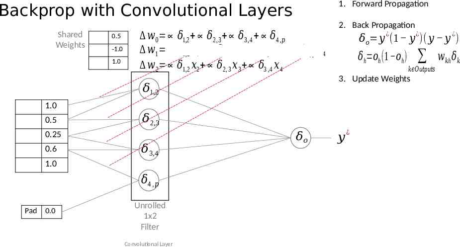
1. Forward Propagation Backprop with Convolutional Layers Shared Weights 0.5 -1.0 1.0 𝑤 0 𝛿1,2 𝛿2,3 𝛿3,4 𝛿4 ,𝑝 𝑤1 𝛿1,2 𝑥 1 𝛿2 , 3 𝑥 2 𝛿3, 4 𝑥 3 𝛿4, 𝑝 𝑥 4 𝑤 2 𝛿1,2 𝑥2 𝛿2, 3 𝑥 3 𝛿3 ,4 𝑥 4 2. Back Propagation 𝛿𝑜 𝑦 (1 𝑦 )( 𝑦 𝑦 ) ¿ 𝛿h 𝑜h (1 𝑜h ) 1.0 𝛿2,3 0.25 0.6 𝛿3,4 1.0 𝛿4 , 𝑝 Pad 0.0 Unrolled 1x2 Filter Convolutional Layer 𝛿𝑜 𝑘𝜖𝑂𝑢𝑡𝑝𝑢𝑡𝑠 3. Update Weights 𝛿1,2 0.5 ¿ 𝑦 ¿ ¿ 𝑤𝑘h 𝛿𝑘
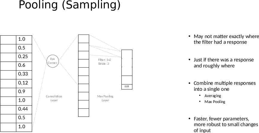
Pooling (Sampling) May not matter exactly where the filter had a response 1.0 0.5 0.25 0.6 Eye Corner Just if there was a response and roughly where Filter: 1x2 Stride: 2 0.33 0.12 0.05 0.9 1.0 Convolution Layer Max Pooling Layer Combine multiple responses into a single one Averaging Max Pooling 0.44 0.5 1.0 Faster, fewer parameters, more robust to small changes of input
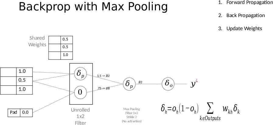
1. Forward Propagation Backprop with Max Pooling 2. Back Propagation 3. Update Weights Shared Weights 0.5 0.5 1.0 1.0 0.5 1.0 Pad 0.0 𝛿𝑝 0 Unrolled 1x2 Filter 1.5 - .82 .75 - .68 𝛿𝑝 .82 Max Pooling Filter 1x2 Stride 2 (No activation) 𝛿𝑜 𝑦 ¿ 𝛿h 𝑜h (1 𝑜h ) 𝑘𝜖𝑂𝑢𝑡𝑝𝑢𝑡𝑠 𝑤𝑘h 𝛿𝑘
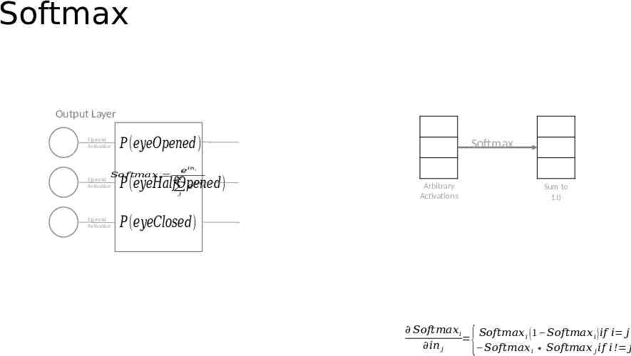
Softmax Output Layer Sigmoid Activation 𝑃 (𝑒𝑦𝑒𝑂𝑝𝑒𝑛𝑒𝑑) 𝑆𝑜𝑓𝑡𝑚𝑎𝑥 𝑖 Sigmoid Activation 𝑖𝑛 𝑖 𝑒 𝑃 (𝑒𝑦𝑒𝐻𝑎𝑙𝑓𝑂𝑝𝑒𝑛𝑒𝑑) 𝑒 𝑁 𝑖𝑛 𝑗 𝑗 Sigmoid Activation Softmax Arbitrary Activations Sum to 1.0 𝑃 (𝑒𝑦𝑒𝐶𝑙𝑜𝑠𝑒𝑑) 𝑆𝑜𝑓𝑡𝑚𝑎𝑥 𝑖 𝑆𝑜𝑓𝑡𝑚𝑎𝑥 𝑖 ( 1 𝑆𝑜𝑓𝑡𝑚𝑎𝑥 𝑖 ) 𝑖𝑓 𝑖 𝑗 𝑖𝑛 𝑗 𝑆𝑜𝑓𝑡𝑚𝑎𝑥 𝑖 𝑆𝑜𝑓𝑡𝑚𝑎𝑥 𝑗 𝑖𝑓 𝑖 ! 𝑗 {
LeNet-5 2d 1d 400 activations 1 output per digit 5x5 Filters Stride 1 No Padding 2x2 Filters Stride 2 Average Pooling http://yann.lecun.com/exdb/publis/pdf/lecun-01a.pdf 1998 paper Sigmoid Activations 60,000 parameters
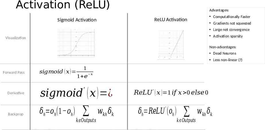
Activation (ReLU) Advantages: Computationally Faster ReLU Activation Sigmoid Activation Gradients not squeezed Large net convergence Activation sparsity Visualization Non-advantages: Dead Neurons Less non-linear (?) Forward Pass Derivative Backprop 𝑠𝑖𝑔𝑚𝑜𝑖𝑑 ( 𝑥 ) 1 𝑥 1 𝑒 ′ 𝑠𝑖𝑔𝑚𝑜𝑖𝑑 ( 𝑥 ) ¿ 𝛿h 𝑜h (1 𝑜h ) 𝑘𝜖𝑂𝑢𝑡𝑝𝑢𝑡𝑠 𝑤𝑘h 𝛿𝑘 𝑅𝑒𝐿𝑈 ′ ( 𝑥 ) 1 𝑖𝑓 𝑥 0 𝑒𝑙𝑠𝑒 0 𝛿h 𝑅𝑒𝐿𝑈 ′ (𝑜h ) 𝑘𝜖 𝑂𝑢𝑡𝑝𝑢𝑡𝑠 𝑤𝑘h 𝛿𝑘
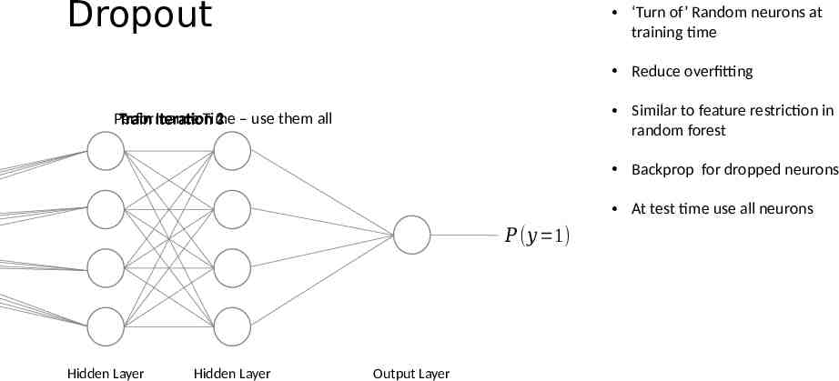
Dropout ‘Turn of’ Random neurons at training time Reduce overfitting Similar to feature restriction in random forest Performance Train Iteration Time 21 – use them all 3 Backprop for dropped neurons At test time use all neurons 𝑃 (𝑦 1) Hidden Layer Hidden Layer Output Layer
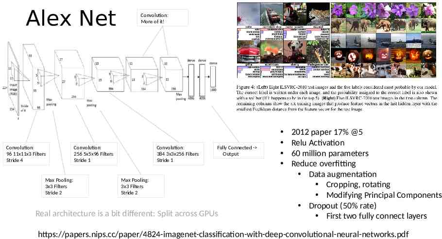
Alex Net Convolution: 96 11x11x3 Filters Stride 4 Max Pooling: 3x3 Filters Stride 2 Convolution: More of it! Convolution: 256 5x5x96 Filters Stride 1 Convolution: 384 3x3x256 Filters Stride 1 Fully Connected - Output Max Pooling: 3x3 Filters Stride 2 Real architecture is a bit different: Split across GPUs 2012 paper 17% @5 Relu Activation 60 million parameters Reduce overfitting Data augmentation Cropping, rotating Modifying Principal Components Dropout (50% rate) First two fully connect layers https://papers.nips.cc/paper/4824-imagenet-classification-with-deep-convolutional-neural-networks.pdf
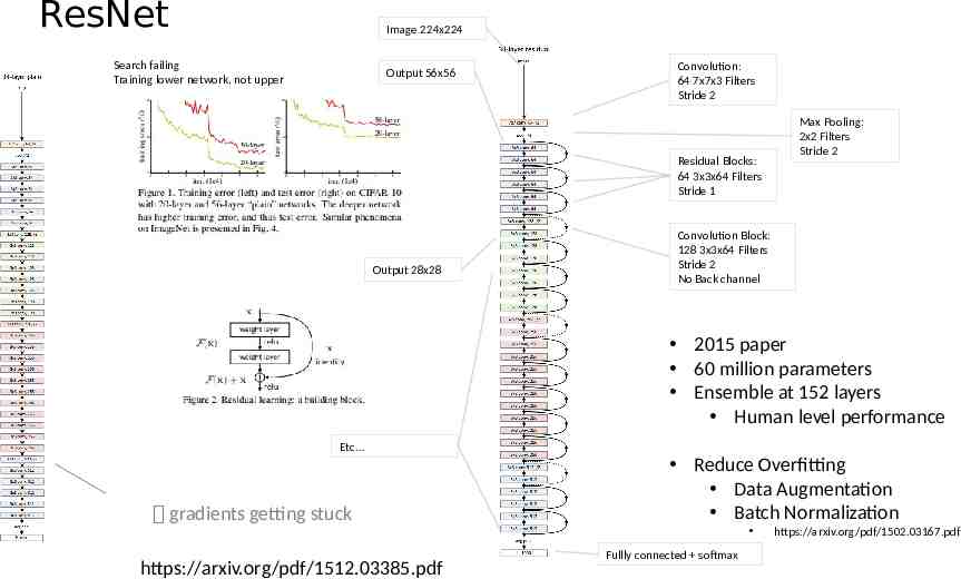
ResNet Image 224x224 Search failing Training lower network, not upper Output 56x56 Convolution: 64 7x7x3 Filters Stride 2 Residual Blocks: 64 3x3x64 Filters Stride 1 Output 28x28 Max Pooling: 2x2 Filters Stride 2 Convolution Block: 128 3x3x64 Filters Stride 2 No Back channel 2015 paper 60 million parameters Ensemble at 152 layers Human level performance Etc gradients getting stuck https://arxiv.org/pdf/1512.03385.pdf Reduce Overfitting Data Augmentation Batch Normalization Fullly connected softmax https://arxiv.org/pdf/1502.03167.pdf
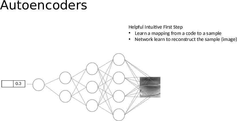
Autoencoders Helpful Intuitive First Step Learn a mapping from a code to a sample Network learn to reconstruct the sample (image) 0.3 0.2 0.1
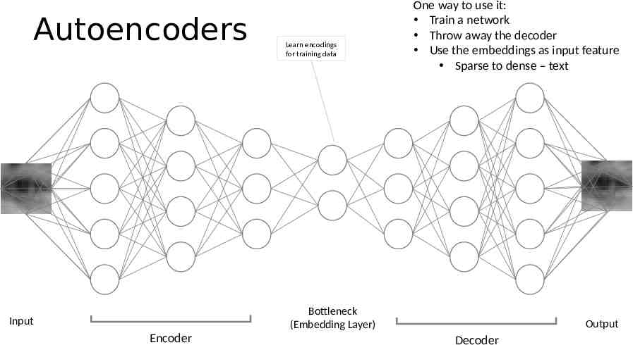
Autoencoders Learn encodings for training data One way to use it: Train a network Throw away the decoder Use the embeddings as input feature Sparse to dense – text Bottleneck (Embedding Layer) Input Encoder Output Decoder
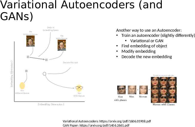
Variational Autoencoders (and GANs) Embedding Dimension 2 Me Without Glasses Delta in Embedding Space Another way to use an Autoencoder: Train an autoencoder (slightly differently) Variational or GAN Find embedding of object Modify embedding Decode the new embedding Me With Glasses Decode this spot Found on several websites: You Without Glasses You With Glasses Embedding Dimension 1 Variational Autoencoders: https://arxiv.org/pdf/1606.05908.pdf GAN Paper: https://arxiv.org/pdf/1406.2661.pdf
Neural Network Architectures/Concepts Fully connected layers Convolutional Layers Recurrent Networks (LSTM & attention) Embeddings Residual Networks MaxPooling Batch Normalization Activation (ReLU) Softmax Dropout Patience
Summary The right network architecture is key to success with neural networks Architecture engineering takes the place of feature engineering Not easy – and things are changing rapidly But if you: Are in a domain with existing architectures Have a lot of data Have GPUs for training Need to chase the best possible accuracies Try Neural Networks