Segmentation by Morphological Watersheds


19 Slides5.23 MB
Segmentation by Morphological Watersheds
Introduction Based on visualizing an image in 3D 25 20 15 10 5 0 100 100 80 50 40 0 imshow(I,[ ]) 20 0 mesh(I) 60
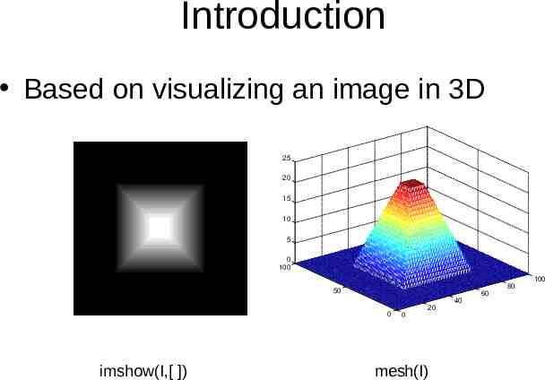
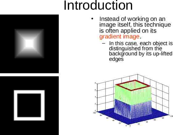
Introduction Instead of working on an image itself, this technique is often applied on its gradient image. – In this case, each object is distinguished from the background by its up-lifted edges 8 6 4 2 0 100 80 100 60 80 60 40 40 20 0 20 0
Basic Definitions I: 2D gray level image DI: Domain of I Path P of length l between p and q in I – A (l 1)-tuple of pixels (p0 p,p1, ,pl q) such that pi,pi 1 are adjacent (4 adjacent, 8 adjacent, or m adjacent, see Section 2.5) l(P): The length of a given path P Minimum – A minimum M of I is a connected plateau of pixels from which it is impossible to reach a point of lower altitude without having to climb
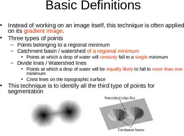
Basic Definitions Instead of working on an image itself, this technique is often applied on its gradient image. Three types of points – Points belonging to a regional minimum – Catchment basin / watershed of a regional minimum Points at which a drop of water will certainly fall to a single minimum – Divide lines / Watershed lines Points at which a drop of water will be equally likely to fall to more than one minimum Crest lines on the topographic surface This technique is to identify all the third type of points for segmentation
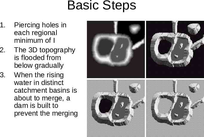
Basic Steps 1. 2. 3. Piercing holes in each regional minimum of I The 3D topography is flooded from below gradually When the rising water in distinct catchment basins is about to merge, a dam is built to prevent the merging
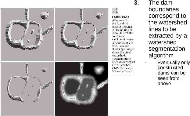
3. The dam boundaries correspond to the watershed lines to be extracted by a watershed segmentation algorithm - Eventually only constructed dams can be seen from above
Dam Construction Based on binary morphological dilation At each step of the algorithm, the binary image in obtained in the following manner 1. Initially, the set of pixels with minimum gray level are 1, others 0. 2. In each subsequent step, we flood the 3D topography from below and the pixels covered by the rising water are 1s and others 0s. (See previous slides)
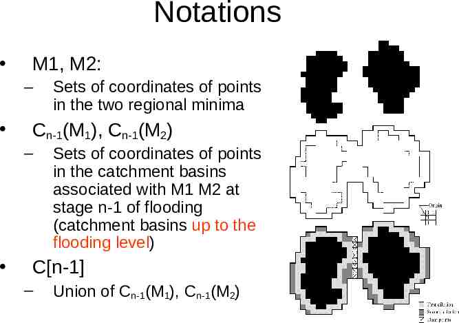
Notations M1, M2: – Cn-1(M1), Cn-1(M2) – Sets of coordinates of points in the two regional minima Sets of coordinates of points in the catchment basins associated with M1 M2 at stage n-1 of flooding (catchment basins up to the flooding level) C[n-1] – Union of Cn-1(M1), Cn-1(M2)
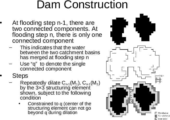
Dam Construction At flooding step n-1, there are two connected components. At flooding step n, there is only one connected component – – This indicates that the water between the two catchment basins has merged at flooding step n Use “q” to denote the single connected component Steps – Repeatedly dilate Cn-1(M1), Cn-1(M2) by the 3 3 structuring element shown, subject to the following condition Constrained to q (center of the structuring element can not go beyond q during dilation
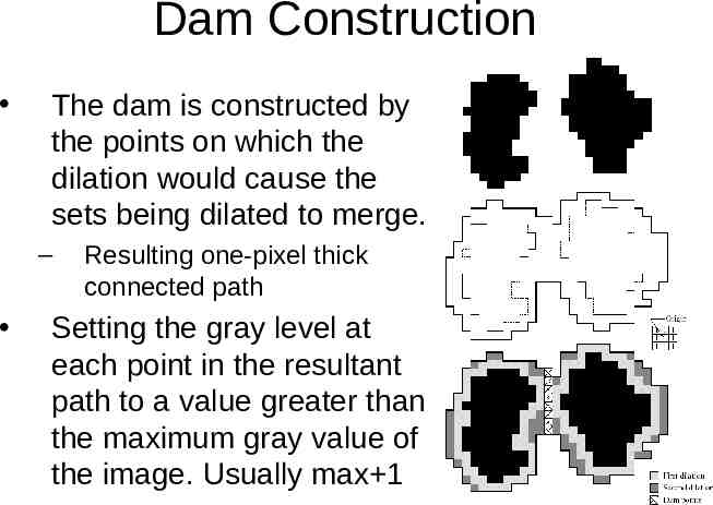
Dam Construction The dam is constructed by the points on which the dilation would cause the sets being dilated to merge. – Resulting one-pixel thick connected path Setting the gray level at each point in the resultant path to a value greater than the maximum gray value of the image. Usually max 1
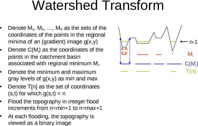
Watershed Transform Denote M1, M2, , MR as the sets of the coordinates of the points in the regional minima of an (gradient) image g(x,y) Denote C(Mi) as the coordinates of the points in the catchment basin associated with regional minimum Mi. Denote the minimum and maximum gray levels of g(x,y) as min and max Denote T[n] as the set of coordinates (s,t) for which g(s,t) n Flood the topography in integer flood increments from n min 1 to n max 1 At each flooding, the topography is viewed as a binary image n-1 Mi C(Mi) T(n)
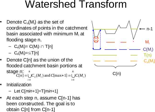
Watershed Transform Denote Cn(Mi) as the set of coordinates of points in the catchment basin associated with minimum Mi at flooding stage n. n-1 Mi – Cn(Mi) C(Mi) T[n] – Cn(Mi) T[n] Denote C[n] as the union of the flooded catchment basin portions at R stage n: R C[n] Cn ( M i ) and C[max 1] C ( M i ) i 1 i 1 Initialization – Let C[min 1] T[min 1] At each step n, assume C[n-1] has been constructed. The goal is to obtain C[n] from C[n-1] C(Mi) T(n) Cn(Mi) C(n)
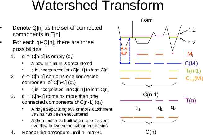
Watershed Transform Dam Denote Q[n] as the set of connected components in T[n]. For each q Q[n], there are three possibilities 1. C(Mi) T(n-1) Cn-1(Mi) A new minimum is encountered q is incorporated into C[n-1] to form C[n] q is incorporated into C[n-1] to form C[n] q C[n-1] contains more than one connected components of C[n-1] (q3) 4. Mi q C[n-1] contains one connected component of C[n-1] (q2) 3. n-2 q C[n-1] is empty (q1) 2. n-1 A ridge separating two or more catchment basins has been encountered A dam has to be built within q to prevent overflow between the catchment basins Repeat the procedure until n max 1 C(n-1) q3 q1 C(n) T(n) q2
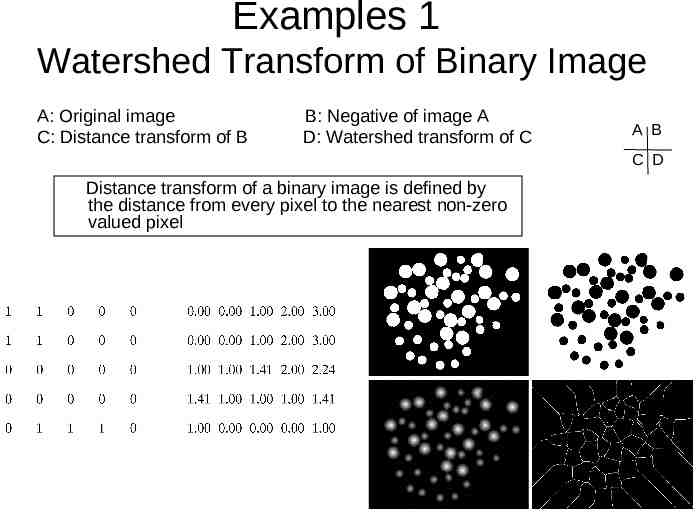
Examples 1 Watershed Transform of Binary Image A: Original image C: Distance transform of B B: Negative of image A D: Watershed transform of C A B C D Distance transform of a binary image is defined by the distance from every pixel to the nearest non-zero valued pixel
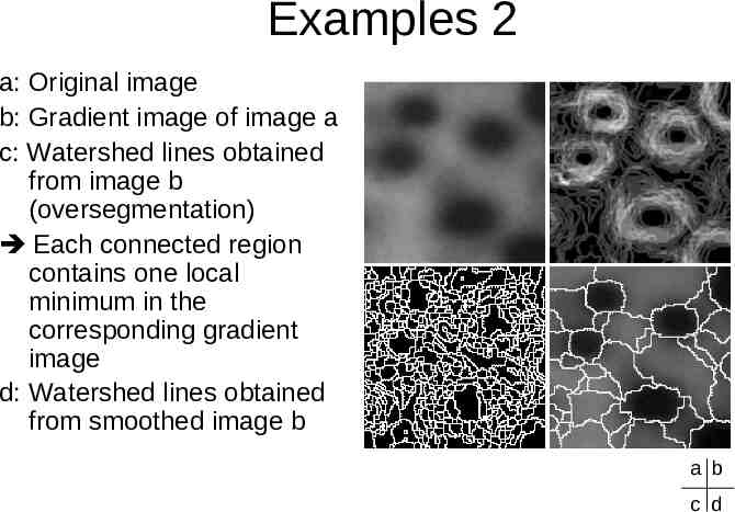
Examples 2 a: Original image b: Gradient image of image a c: Watershed lines obtained from image b (oversegmentation) Each connected region contains one local minimum in the corresponding gradient image d: Watershed lines obtained from smoothed image b a b c d
The Use of Markers Internal markers are used to limit the number of regions by specifying the objects of interest – – – Like seeds in region growing method Can be assigned manually or automatically Regions without markers are allowed to be merged (no dam is to be built) External markers those pixels we are confident to belong to the background – Watershed lines are typical external markers and they belong the same (background) region
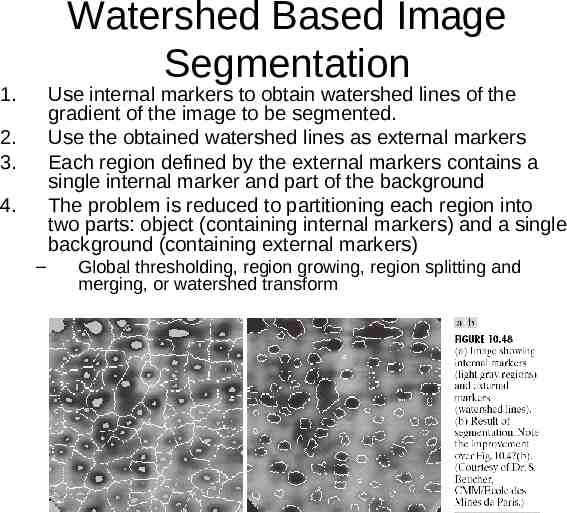
Watershed Based Image Segmentation 1. Use internal markers to obtain watershed lines of the gradient of the image to be segmented. Use the obtained watershed lines as external markers Each region defined by the external markers contains a single internal marker and part of the background The problem is reduced to partitioning each region into two parts: object (containing internal markers) and a single background (containing external markers) 2. 3. 4. – Global thresholding, region growing, region splitting and merging, or watershed transform
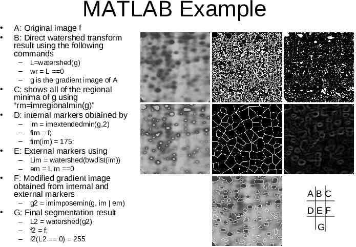
MATLAB Example A: Original image f B: Direct watershed transform result using the following commands – – – C: shows all of the regional minima of g using “rm imregionalmin(g)” D: internal markers obtained by – – – Lim watershed(bwdist(im)) em Lim 0 F: Modified gradient image obtained from internal and external markers – im imextendedmin(g,2) fim f; fim(im) 175; E: External markers using – – L watershed(g) wr L 0 g is the gradient image of A g2 imimposemin(g, im em) G: Final segmentation result – – – L2 watershed(g2) f2 f; f2(L2 0) 255 ABC DEF G