Matching Supply with Demand: An Introduction to Operations Management

20 Slides230.50 KB
Matching Supply with Demand: An Introduction to Operations Management Gérard Cachon ChristianTerwiesch All slides in this file are copyrighted by Gerard Cachon and Christian Terwiesch. Any instructor that adopts Matching Supply with Demand: An Introduction to Operations Management as a required text for their course is free to use and modify these slides as desired. All others must obtain explicit written permission from the authors to use these slides. Slide 1
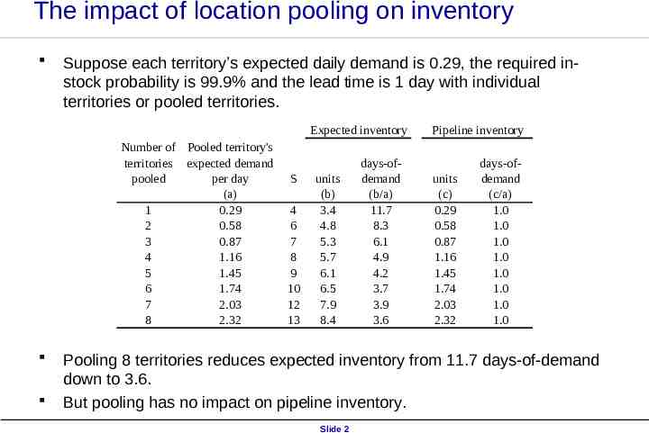
The impact of location pooling on inventory Suppose each territory’s expected daily demand is 0.29, the required instock probability is 99.9% and the lead time is 1 day with individual territories or pooled territories. Expected inventory Number of Pooled territory's territories expected demand pooled per day (a) 1 0.29 2 0.58 3 0.87 4 1.16 5 1.45 6 1.74 7 2.03 8 2.32 S 4 6 7 8 9 10 12 13 units (b) 3.4 4.8 5.3 5.7 6.1 6.5 7.9 8.4 days-ofdemand (b/a) 11.7 8.3 6.1 4.9 4.2 3.7 3.9 3.6 Pipeline inventory units (c) 0.29 0.58 0.87 1.16 1.45 1.74 2.03 2.32 days-ofdemand (c/a) 1.0 1.0 1.0 1.0 1.0 1.0 1.0 1.0 Pooling 8 territories reduces expected inventory from 11.7 days-of-demand down to 3.6. But pooling has no impact on pipeline inventory. Slide 2
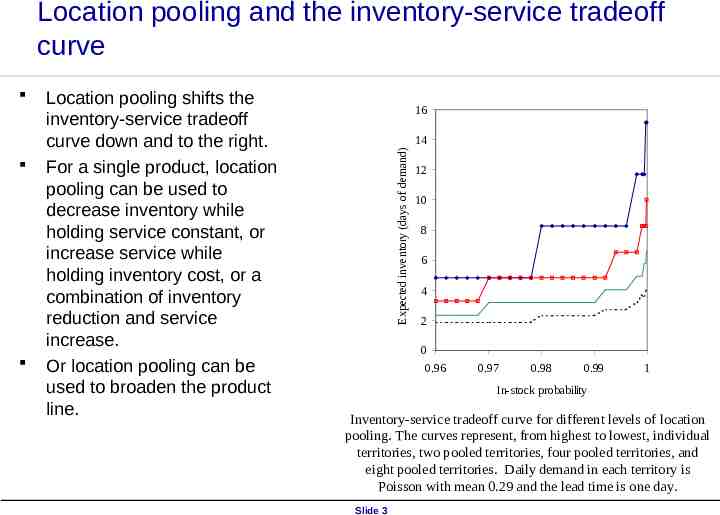
Location pooling and the inventory-service tradeoff curve Location pooling shifts the inventory-service tradeoff curve down and to the right. For a single product, location pooling can be used to decrease inventory while holding service constant, or increase service while holding inventory cost, or a combination of inventory reduction and service increase. Or location pooling can be used to broaden the product line. 16 14 Expected inventory (days of demand) 12 10 8 6 4 2 0 0.96 0.97 0.98 0.99 1 In-stock probability Inventory-service tradeoff curve for different levels of location pooling. The curves represent, from highest to lowest, individual territories, two pooled territories, four pooled territories, and eight pooled territories. Daily demand in each territory is Poisson with mean 0.29 and the lead time is one day. Slide 3
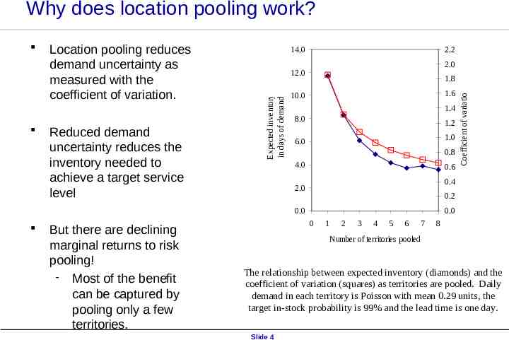
Why does location pooling work? Reduced demand uncertainty reduces the inventory needed to achieve a target service level 14.0 2.2 2.0 12.0 1.8 1.6 10.0 1.4 8.0 1.2 1.0 6.0 0.8 4.0 0.6 0.4 2.0 0.2 0.0 But there are declining marginal returns to risk pooling! Most of the benefit can be captured by pooling only a few territories. Coefficient of variation Location pooling reduces demand uncertainty as measured with the coefficient of variation. Expected inventory in days of demand 0.0 0 1 2 3 4 5 6 7 8 Number of territories pooled The relationship between expected inventory (diamonds) and the coefficient of variation (squares) as territories are pooled. Daily demand in each territory is Poisson with mean 0.29 units, the target in-stock probability is 99% and the lead time is one day. Slide 4
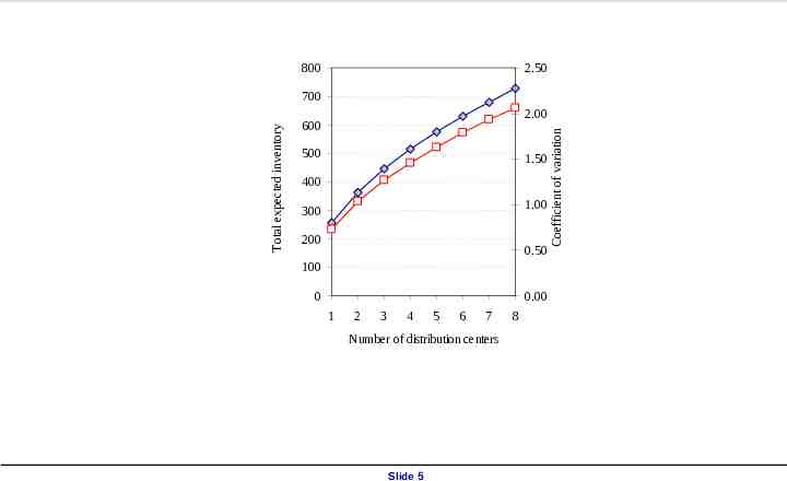
800 2.50 2.00 600 500 1.50 400 1.00 300 200 0.50 100 0 0.00 1 2 3 4 5 6 7 Number of distribution centers Slide 5 8 Coefficient of variation Total expected inventory 700
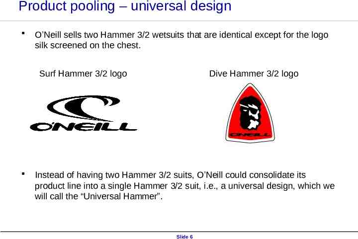
Product pooling – universal design O’Neill sells two Hammer 3/2 wetsuits that are identical except for the logo silk screened on the chest. Surf Hammer 3/2 logo Dive Hammer 3/2 logo Instead of having two Hammer 3/2 suits, O’Neill could consolidate its product line into a single Hammer 3/2 suit, i.e., a universal design, which we will call the “Universal Hammer”. Slide 6
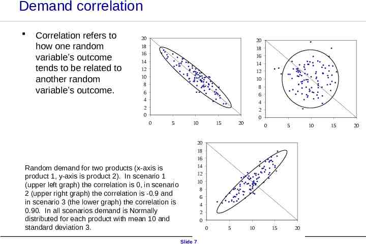
Demand correlation Correlation refers to how one random variable’s outcome tends to be related to another random variable’s outcome. 20 18 16 14 12 10 8 6 4 2 0 0 5 10 15 20 18 16 14 12 10 8 6 4 2 0 20 0 5 10 20 18 16 14 12 10 8 6 4 2 0 Random demand for two products (x-axis is product 1, y-axis is product 2). In scenario 1 (upper left graph) the correlation is 0, in scenario 2 (upper right graph) the correlation is -0.9 and in scenario 3 (the lower graph) the correlation is 0.90. In all scenarios demand is Normally distributed for each product with mean 10 and standard deviation 3. 0 Slide 7 5 10 15 20 15 20
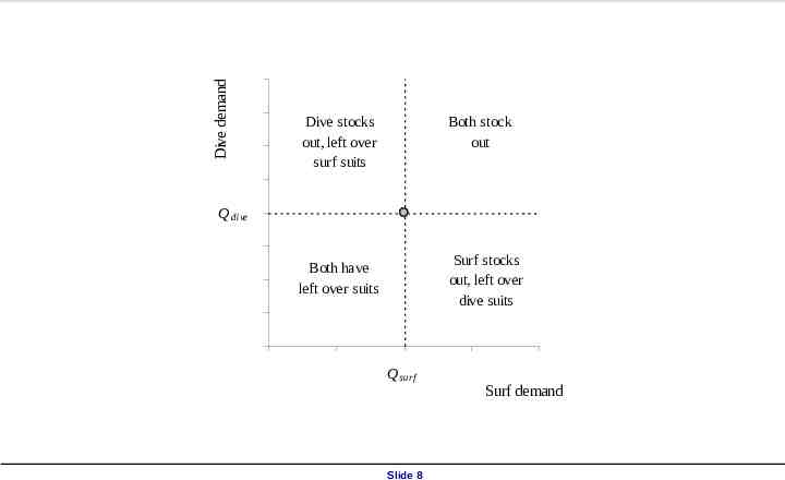
Dive demand Dive stocks out, left over surf suits Both stock out Q dive Surf stocks out, left over dive suits Both have left over suits Q surf Slide 8 Surf demand
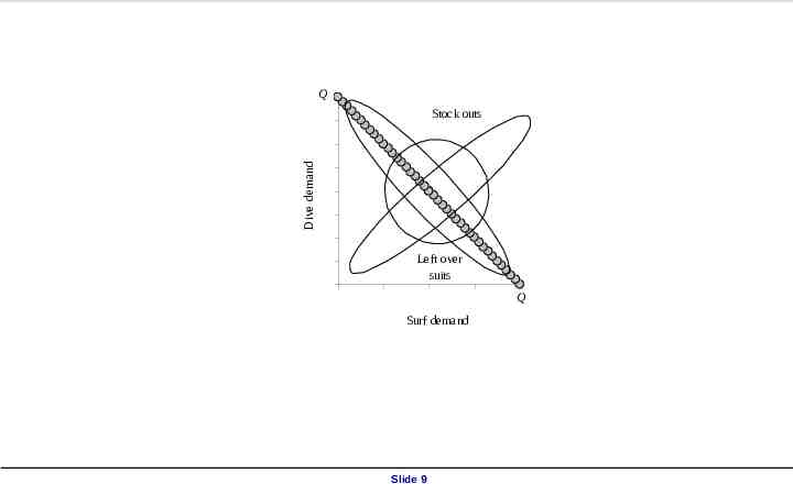
Q Dive demand Stock outs Left over suits Q Surf demand Slide 9
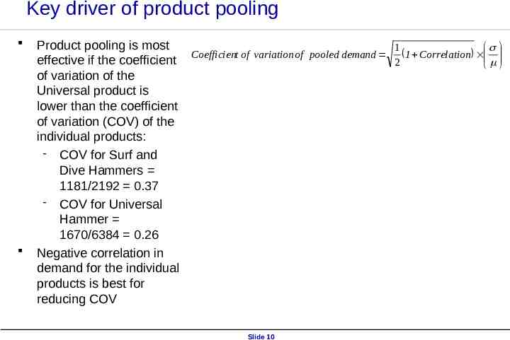
Key driver of product pooling Coefficient of variation Product pooling is most 1 Coefficient of variation of pooled demand 1 Correlation effective if the coefficient 2 of variation of the 450000 0.40 Universal product is lower than the coefficient 0.35 440000 of variation (COV) of the 0.30 430000 individual products: 0.25 COV for Surf and 420000 0.20 Dive Hammers 410000 1181/2192 0.37 0.15 400000 COV for Universal 0.10 Hammer 390000 0.05 1670/6384 0.26 380000 0.00 Negative correlation in -1 -0.5 0 0.5 1 demand for the individual Correlation products is best for The correlation between surf and dive demand for the Hammer 3/2 and reducing COV Expected profit the expected profit of the universal Hammer wetsuit (decreasing curve) and the coefficient of variation of total demand (increasing curve) Slide 10
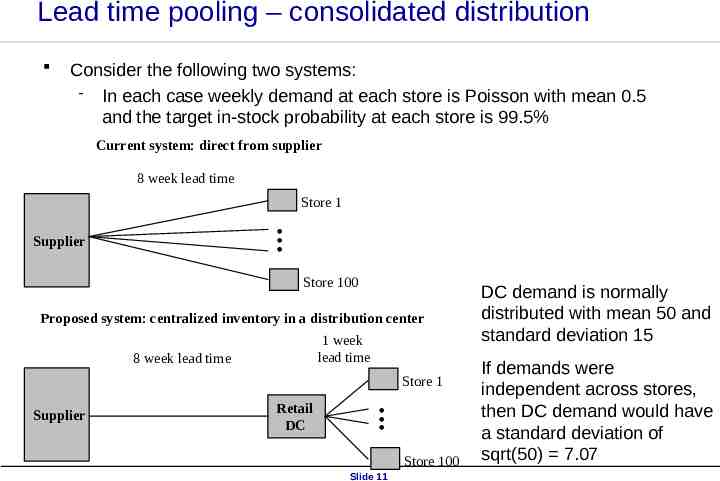
Lead time pooling – consolidated distribution Consider the following two systems: In each case weekly demand at each store is Poisson with mean 0.5 and the target in-stock probability at each store is 99.5% Current system: direct from supplier 8 week lead time . . Supplier Store 1 Store 100 Proposed system: centralized inventory in a distribution center 1 week lead time 8 week lead time Supplier Retail DC . . Store 1 Store 100 Slide 11 DC demand is normally distributed with mean 50 and standard deviation 15 If demands were independent across stores, then DC demand would have a standard deviation of sqrt(50) 7.07
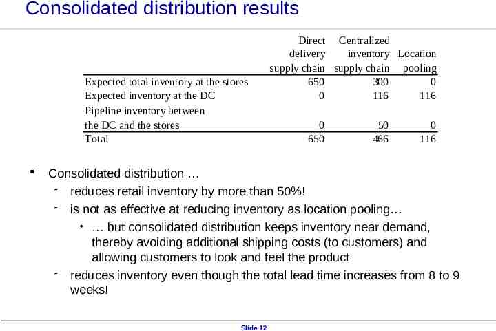
Consolidated distribution results Expected total inventory at the stores Expected inventory at the DC Pipeline inventory between the DC and the stores Total Direct Centralized delivery inventory Location supply chain supply chain pooling 650 300 0 0 116 116 0 650 50 466 0 116 Consolidated distribution reduces retail inventory by more than 50%! is not as effective at reducing inventory as location pooling but consolidated distribution keeps inventory near demand, thereby avoiding additional shipping costs (to customers) and allowing customers to look and feel the product reduces inventory even though the total lead time increases from 8 to 9 weeks! Slide 12
1000 900 Inventory (units) 800 700 600 500 400 300 200 100 0 0 10 20 30 40 50 60 70 Standard deviation of weekly demand across all stores Slide 13
700 Inventory (units) 600 500 400 300 200 1 2 3 4 5 6 7 Lead time from supplier (in weeks) Slide 14 8
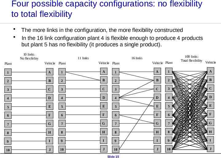
Four possible capacity configurations: no flexibility to total flexibility The more links in the configuration, the more flexibility constructed In the 16 link configuration plant 4 is flexible enough to produce 4 products but plant 5 has no flexibility (it produces a single product). 10 links: No flexibility Plant 11 links Vehicle Plant 16 links Vehicle Plant Vehicle Plant 100 links: Total flexibility Vehicle 1 A 1 A 1 A 1 A 2 B 2 B 2 B 2 B 3 C 3 C 3 C 3 C 4 D 4 D 4 D 4 D 5 E 5 E 5 E 5 E 6 F 6 F 6 F 6 F 7 G 7 G 7 G 7 G 8 H 8 H 8 H 8 H 9 I 9 I 9 I 9 I 10 J 10 J 10 J 10 J Slide 15
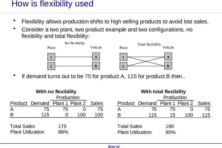
How is flexibility used Flexibility allows production shifts to high selling products to avoid lost sales. Consider a two plant, two product example and two configurations, no flexibility and total flexibility: No flexibility Total flexibility Plant Vehicle Plant Vehicle 1 A 1 A 2 B 2 B If demand turns out to be 75 for product A, 115 for product B then. With no flexibility Production Product Demand Plant 1 Plant 2 Sales A 75 75 0 75 B 115 0 100 100 With total flexibility Production Product Demand Plant 1 Plant 2 A 75 75 0 B 115 15 100 Total Sales Plant Utilization Total Sales Plant Utilization 175 88% Slide 16 190 95% Sales 75 115
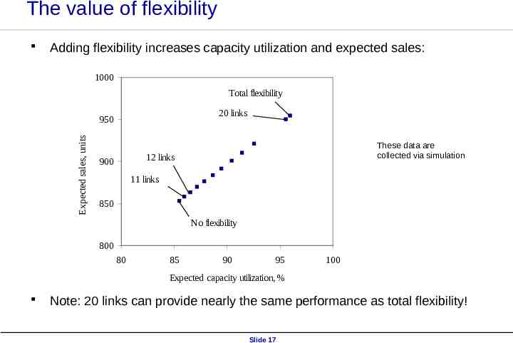
The value of flexibility Adding flexibility increases capacity utilization and expected sales: 1000 Total flexibility 20 links Expected sales, units 950 These data are collected via simulation 12 links 900 11 links 850 No flexibility 800 80 85 90 95 100 Expected capacity utilization, % Note: 20 links can provide nearly the same performance as total flexibility! Slide 17
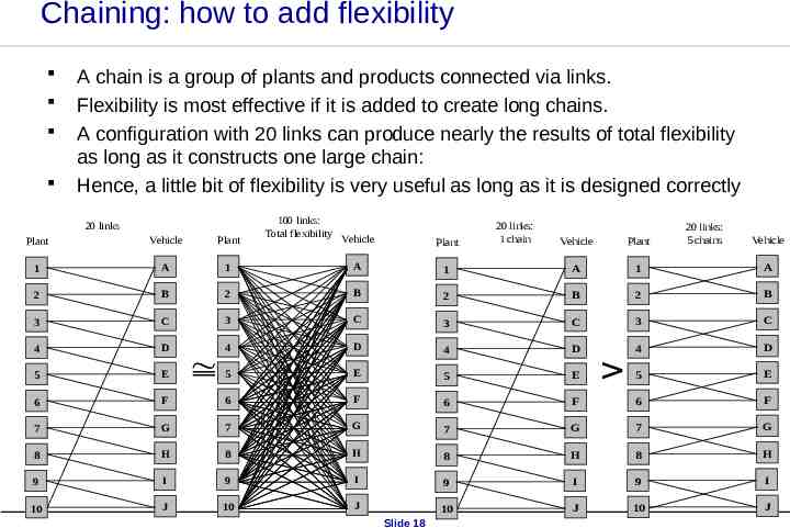
Chaining: how to add flexibility A chain is a group of plants and products connected via links. Flexibility is most effective if it is added to create long chains. A configuration with 20 links can produce nearly the results of total flexibility as long as it constructs one large chain: Hence, a little bit of flexibility is very useful as long as it is designed correctly 20 links 100 links: Total flexibility Vehicle Plant Plant Vehicle Plant 1 A 1 A 2 B 2 3 C 4 D 5 E 6 20 links: 1 chain 20 links: 5 chains Vehicle Vehicle Plant 1 A 1 A B 2 B 2 B 3 C 3 C 3 C 4 D 4 D 4 D 5 E 5 E 5 E F 6 F 6 F 6 F 7 G 7 G 7 G 7 G 8 H 8 H 8 H 8 H 9 I 9 I 9 I 9 I 10 J 10 J 10 J 10 J Slide 18
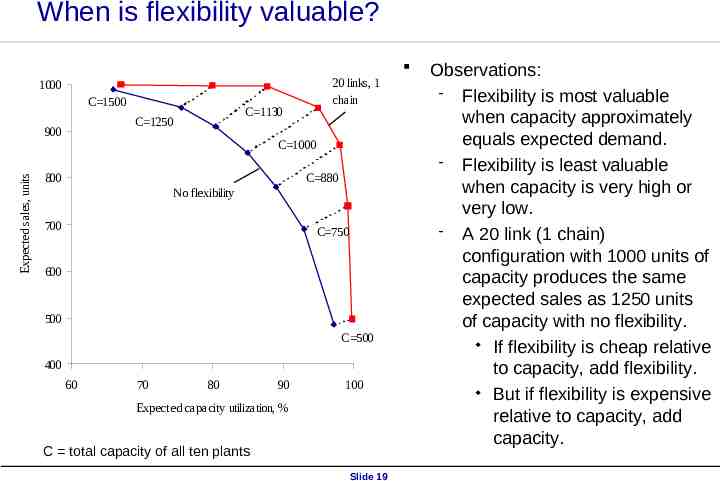
When is flexibility valuable? 20 links, 1 chain 1000 C 1500 900 Expected sales, units C 1130 C 1250 C 1000 800 C 880 No flexibility 700 C 750 600 500 C 500 400 60 70 80 90 100 Expected capacity utilization, % C total capacity of all ten plants Slide 19 Observations: Flexibility is most valuable when capacity approximately equals expected demand. Flexibility is least valuable when capacity is very high or very low. A 20 link (1 chain) configuration with 1000 units of capacity produces the same expected sales as 1250 units of capacity with no flexibility. If flexibility is cheap relative to capacity, add flexibility. But if flexibility is expensive relative to capacity, add capacity.
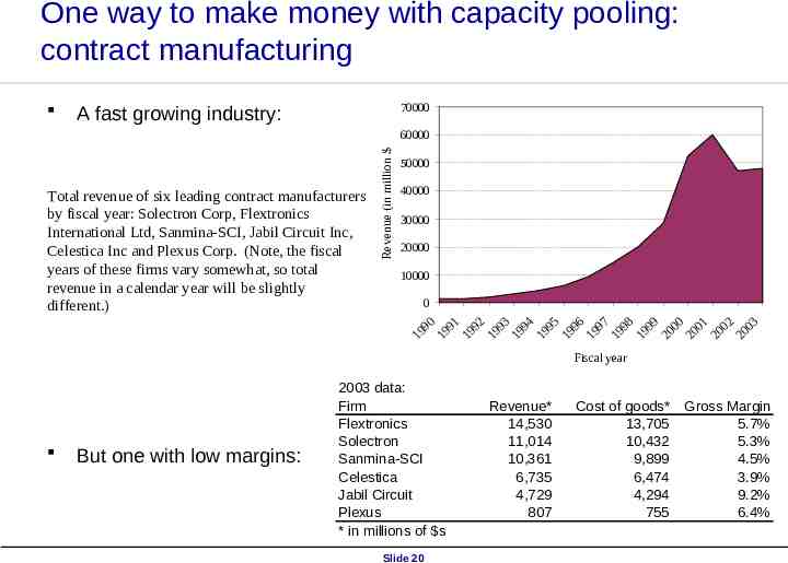
One way to make money with capacity pooling: contract manufacturing 70000 A fast growing industry: 60000 50000 40000 30000 20000 10000 0 19 90 19 91 19 92 19 93 19 94 19 95 19 96 19 97 19 98 19 99 20 00 20 01 20 02 20 03 Total revenue of six leading contract manufacturers by fiscal year: Solectron Corp, Flextronics International Ltd, Sanmina-SCI, Jabil Circuit Inc, Celestica Inc and Plexus Corp. (Note, the fiscal years of these firms vary somewhat, so total revenue in a calendar year will be slightly different.) Revenue (in million s) Fiscal year But one with low margins: 2003 data: Firm Flextronics Solectron Sanmina-SCI Celestica Jabil Circuit Plexus * in millions of s Slide 20 Revenue* 14,530 11,014 10,361 6,735 4,729 807 Cost of goods* 13,705 10,432 9,899 6,474 4,294 755 Gross Margin 5.7% 5.3% 4.5% 3.9% 9.2% 6.4%