Introduction to Algorithms 6.046J Lecture 1 Prof. Shafi


54 Slides293.50 KB
Introduction to Algorithms 6.046J Lecture 1 Prof. Shafi Goldwasser Prof. Erik Demaine
Welcome to Introduction to Algorithms, Spring 2004 Handouts 1. 2. 3. 4. Course Information Course Calendar Problem Set 1 Akra-Bazzi Handout L1.2
Course information 1. 2. 3. 4. 5. 6. Staff Prerequisites Lectures & Recitations Handouts Textbook (CLRS) Website 8. Extra Help 9. Registration 10.Problem sets 11.Describing algorithms 12.Grading policy 13.Collaboration policy L1.3
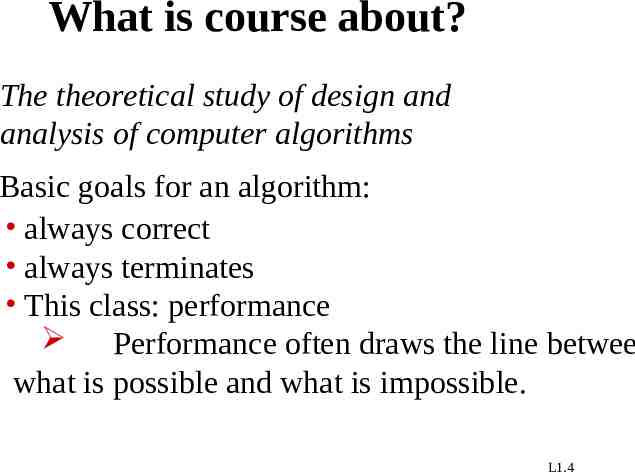
What is course about? The theoretical study of design and analysis of computer algorithms Basic goals for an algorithm: always correct always terminates This class: performance Performance often draws the line betwee what is possible and what is impossible. L1.4
Design and Analysis of Algorithms Analysis: predict the cost of an algorithm in terms of resources and performance Design: design algorithms which minimize the cost L1.5
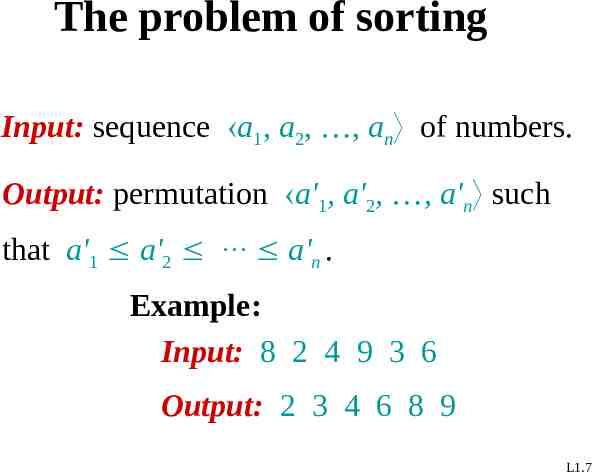
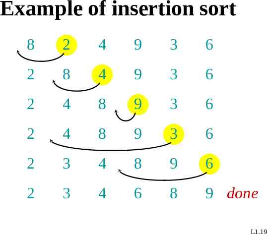
The problem of sorting Input: sequence a1, a2, , an of numbers. Output: permutation a'1, a'2, , a'n such that a'1 a'2 a'n . Example: Input: 8 2 4 9 3 6 Output: 2 3 4 6 8 9 L1.7
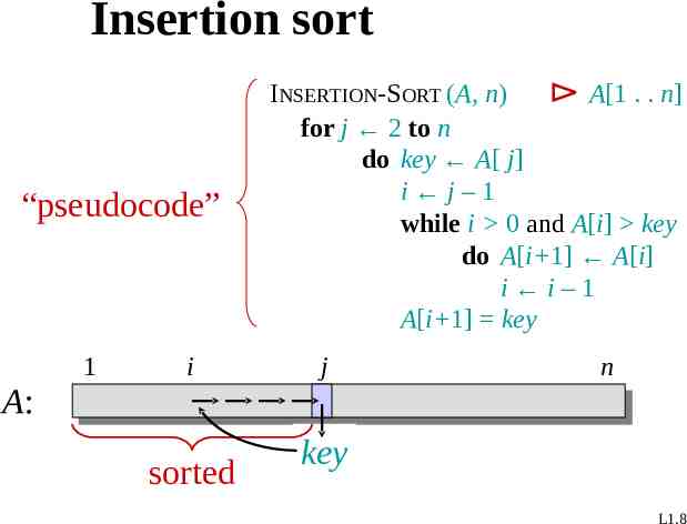
Insertion sort “pseudocode” 1 i INSERTION-SORT (A, n) A[1 . . n] for j 2 to n do key A[ j] i j–1 while i 0 and A[i] key do A[i 1] A[i] i i–1 A[i 1] key j n A: sorted key L1.8
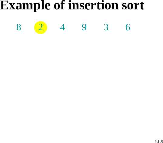
Example of insertion sort 8 2 4 9 3 6 L1.9
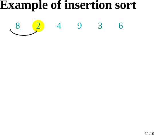
Example of insertion sort 8 2 4 9 3 6 L1.10
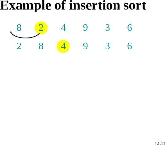
Example of insertion sort 8 2 4 9 3 6 2 8 4 9 3 6 L1.11
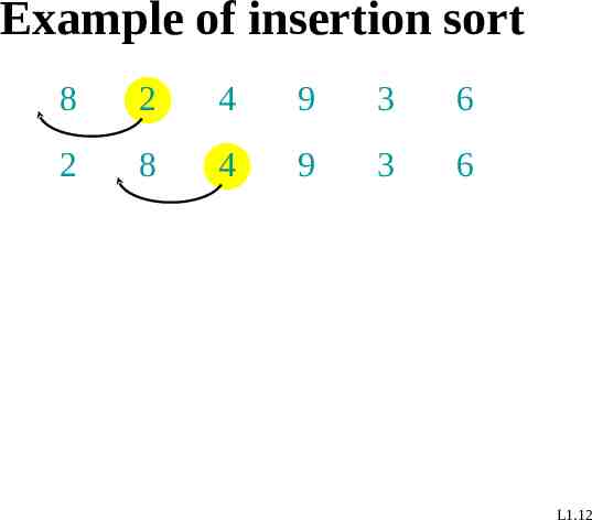
Example of insertion sort 8 2 4 9 3 6 2 8 4 9 3 6 L1.12
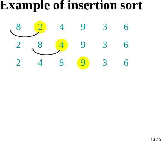
Example of insertion sort 8 2 4 9 3 6 2 8 4 9 3 6 2 4 8 9 3 6 L1.13
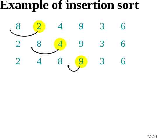
Example of insertion sort 8 2 4 9 3 6 2 8 4 9 3 6 2 4 8 9 3 6 L1.14
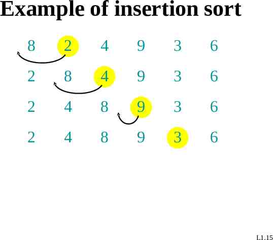
Example of insertion sort 8 2 4 9 3 6 2 8 4 9 3 6 2 4 8 9 3 6 2 4 8 9 3 6 L1.15
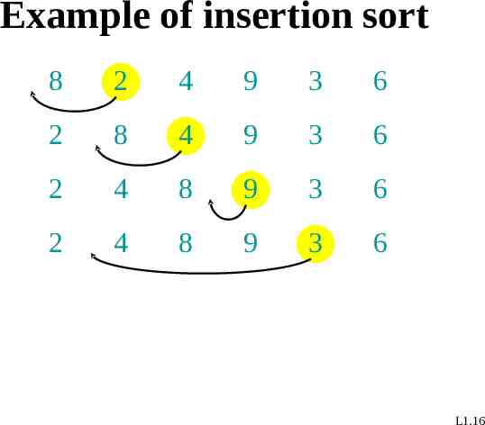
Example of insertion sort 8 2 4 9 3 6 2 8 4 9 3 6 2 4 8 9 3 6 2 4 8 9 3 6 L1.16
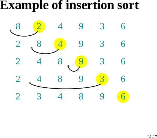
Example of insertion sort 8 2 4 9 3 6 2 8 4 9 3 6 2 4 8 9 3 6 2 4 8 9 3 6 2 3 4 8 9 6 L1.17
Example of insertion sort 8 2 4 9 3 6 2 8 4 9 3 6 2 4 8 9 3 6 2 4 8 9 3 6 2 3 4 8 9 6 L1.18
Example of insertion sort 8 2 4 9 3 6 2 8 4 9 3 6 2 4 8 9 3 6 2 4 8 9 3 6 2 3 4 8 9 6 2 3 4 6 8 9 done L1.19
Running time The running time depends on the input: an already sorted sequence is easier to sort. Major Simplifying Convention: Parameterize the running time by the size of the input, since short sequences are easier to sort than long ones. TA(n) time of A on length n inputs Generally, we seek upper bounds on the running time, to have a guarantee of performance. L1.20
Kinds of analyses Worst-case: (usually) T(n) maximum time of algorithm on any input of size n. Average-case: (sometimes) T(n) expected time of algorithm over all inputs of size n. Need assumption of statistical distribution of inputs. Best-case: (NEVER) Cheat with a slow algorithm that works fast on some input. L1.21
Machine-independent time What is insertion sort’s worst-case time? BIG IDEAS: Ignore machine dependent constants, otherwise impossible to verify and to compare algorithms Look at growth of T(n) as n . “Asymptotic Analysis” L1.22
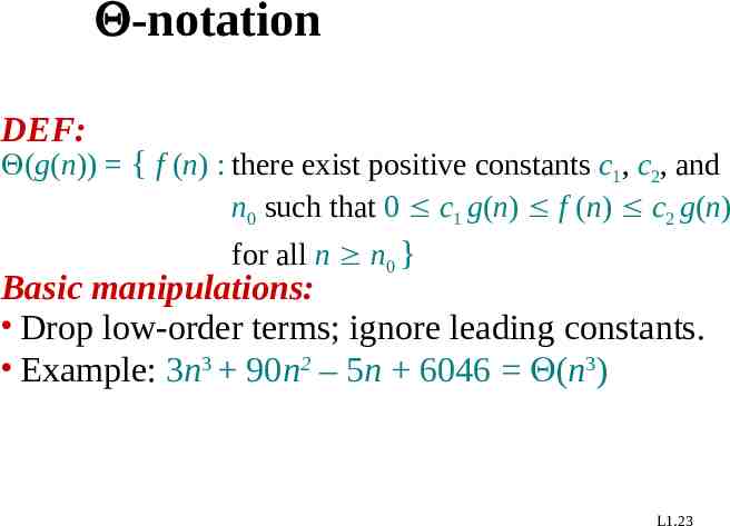
-notation DEF: (g(n)) { f (n) : there exist positive constants c1, c2, and n0 such that 0 c1 g(n) f (n) c2 g(n) for all n n0 } Basic manipulations: Drop low-order terms; ignore leading constants. Example: 3n3 90n2 – 5n 6046 (n3) L1.23
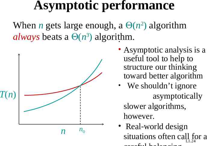
Asymptotic performance When n gets large enough, a (n2) algorithm always beats a (n3) algorithm. . T(n) n n0 Asymptotic analysis is a useful tool to help to structure our thinking toward better algorithm We shouldn’t ignore asymptotically slower algorithms, however. Real-world design situations often callL1.24for a
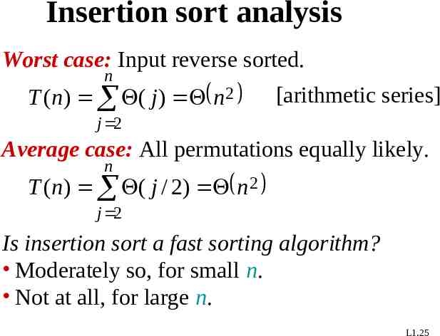
Insertion sort analysis Worst case: Input reverse sorted. n T (n) ( j ) n 2 [arithmetic series] j 2 Average case: All permutations equally likely. n T (n) ( j / 2) n 2 j 2 Is insertion sort a fast sorting algorithm? Moderately so, for small n. Not at all, for large n. L1.25
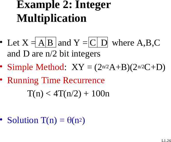
Example 2: Integer Multiplication Let X A B and Y C D where A,B,C and D are n/2 bit integers Simple Method: XY (2n/2A B)(2n/2C D) Running Time Recurrence T(n) 4T(n/2) 100n Solution T(n) (n2) L1.26
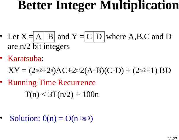
Better Integer Multiplication Let X A B and Y C D where A,B,C and D are n/2 bit integers Karatsuba: XY (2n/2 2n)AC 2n/2(A-B)(C-D) (2n/2 1) BD Running Time Recurrence T(n) 3T(n/2) 100n Solution: (n) O(n log 3) L1.27
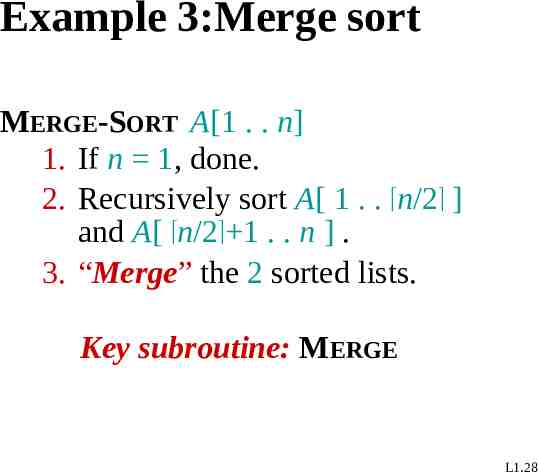
Example 3:Merge sort MERGE-SORT A[1 . . n] 1. If n 1, done. 2. Recursively sort A[ 1 . . n/2 ] and A[ n/2 1 . . n ] . 3. “Merge” the 2 sorted lists. Key subroutine: MERGE L1.28
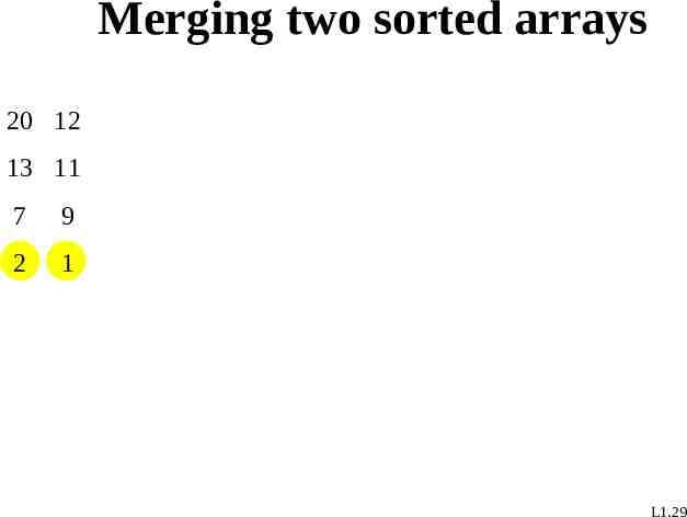
Merging two sorted arrays 20 12 13 11 7 9 2 1 L1.29
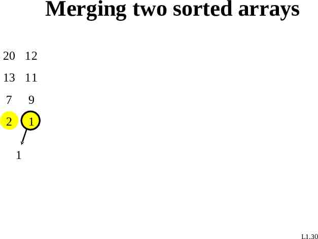
Merging two sorted arrays 20 12 13 11 7 9 2 1 1 L1.30
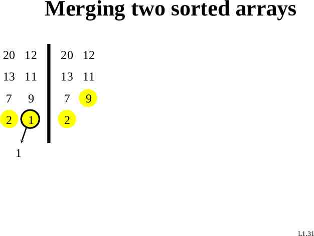
Merging two sorted arrays 20 12 20 12 13 11 13 11 7 9 7 2 1 2 9 1 L1.31
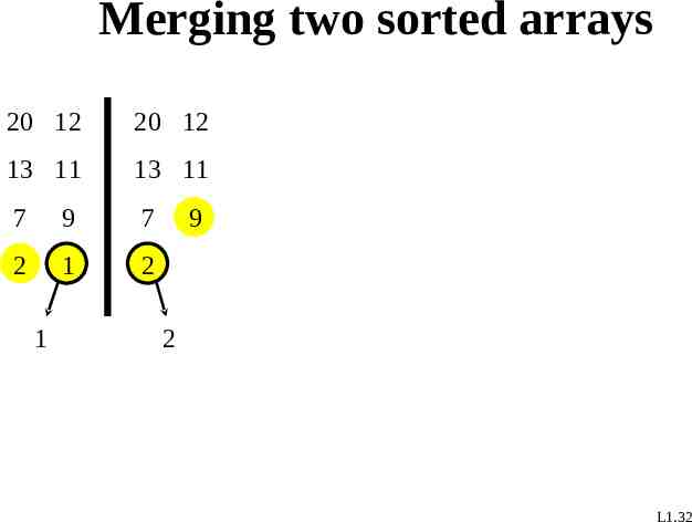
Merging two sorted arrays 20 12 20 12 13 11 13 11 7 9 7 2 1 2 1 9 2 L1.32
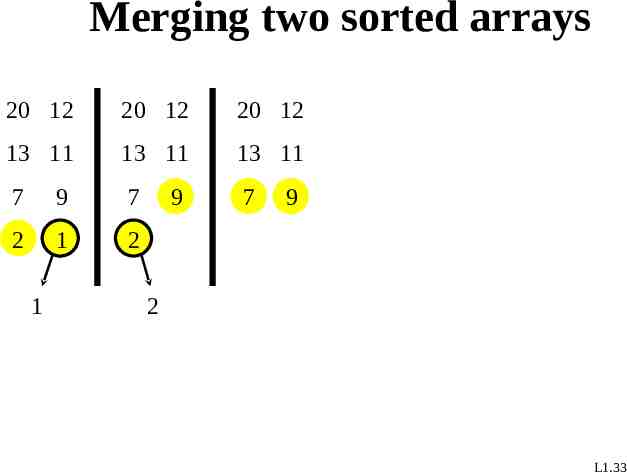
Merging two sorted arrays 20 12 20 12 20 12 13 11 13 11 13 11 7 9 7 7 2 1 2 1 9 9 2 L1.33
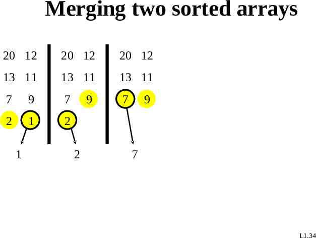
Merging two sorted arrays 20 12 20 12 20 12 13 11 13 11 13 11 7 9 7 7 2 1 2 1 9 2 9 7 L1.34
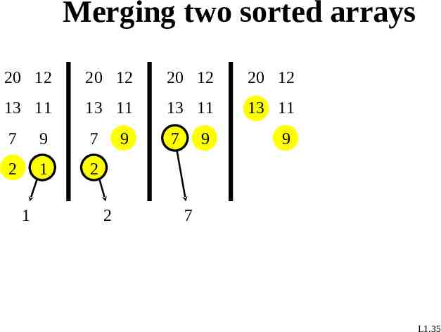
Merging two sorted arrays 20 12 20 12 20 12 20 12 13 11 13 11 13 11 13 11 7 9 7 7 2 1 2 1 9 2 9 9 7 L1.35
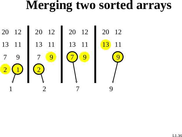
Merging two sorted arrays 20 12 20 12 20 12 20 12 13 11 13 11 13 11 13 11 7 9 7 7 2 1 2 1 9 2 9 7 9 9 L1.36
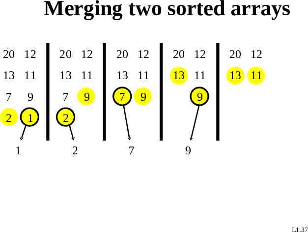
Merging two sorted arrays 20 12 20 12 20 12 20 12 20 12 13 11 13 11 13 11 13 11 13 11 7 9 7 7 2 1 2 1 9 2 9 7 9 9 L1.37
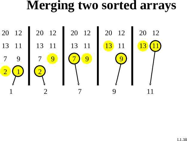
Merging two sorted arrays 20 12 20 12 20 12 20 12 20 12 13 11 13 11 13 11 13 11 13 11 7 9 7 7 2 1 2 1 9 2 9 7 9 9 11 L1.38
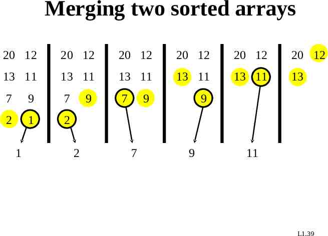
Merging two sorted arrays 20 12 20 12 20 12 20 12 20 12 20 12 13 11 13 11 13 11 13 11 13 11 13 7 9 7 7 2 1 2 1 9 2 9 7 9 9 11 L1.39
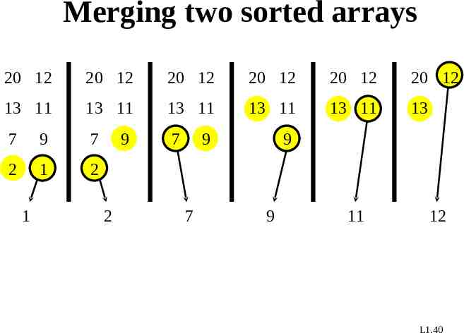
Merging two sorted arrays 20 12 20 12 20 12 20 12 20 12 20 12 13 11 13 11 13 11 13 11 13 11 13 7 9 7 7 2 1 2 1 9 2 9 7 9 9 11 12 L1.40
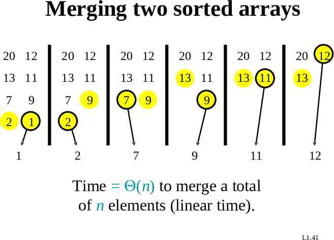
Merging two sorted arrays 20 12 20 12 20 12 20 12 20 12 20 12 13 11 13 11 13 11 13 11 13 11 13 7 9 7 7 2 1 2 1 9 2 9 7 9 9 11 12 Time (n) to merge a total of n elements (linear time). L1.41
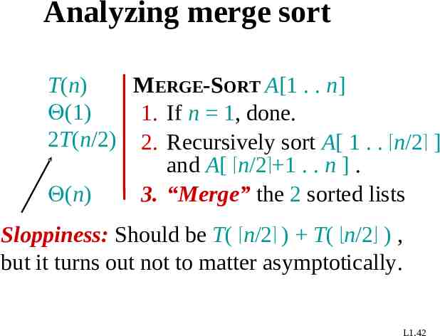
Analyzing merge sort T(n) MERGE-SORT A[1 . . n] (1) 1. If n 1, done. 2T(n/2) 2. Recursively sort A[ 1 . . n/2 ] and A[ n/2 1 . . n ] . 3. “Merge” the 2 sorted lists (n) Sloppiness: Should be T( n/2 ) T( n/2 ) , but it turns out not to matter asymptotically. L1.42
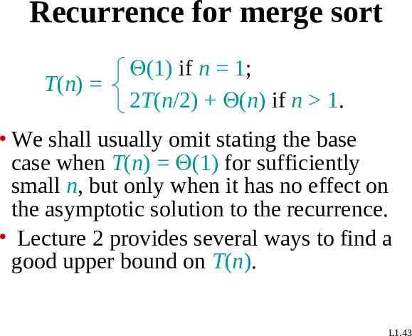
Recurrence for merge sort T(n) (1) if n 1; 2T(n/2) (n) if n 1. We shall usually omit stating the base case when T(n) (1) for sufficiently small n, but only when it has no effect on the asymptotic solution to the recurrence. Lecture 2 provides several ways to find a good upper bound on T(n). L1.43
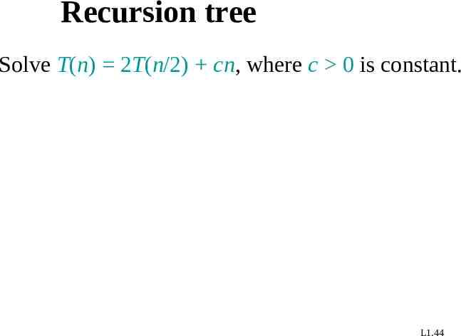
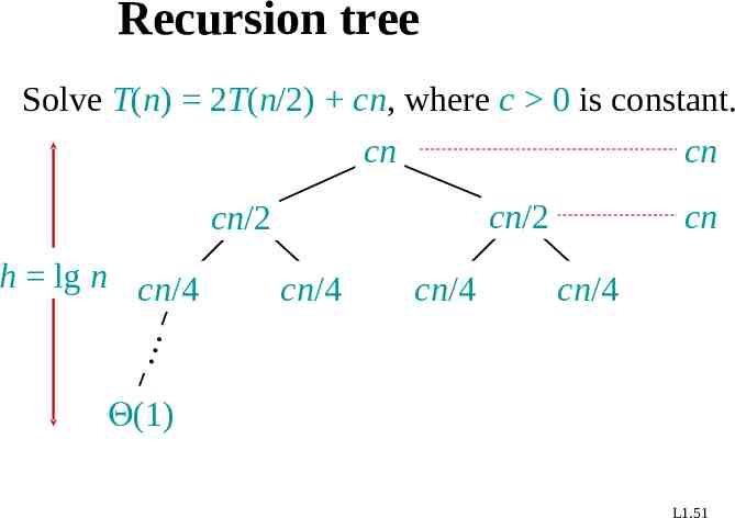
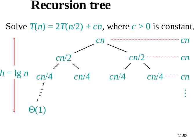
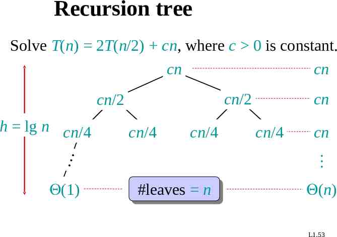
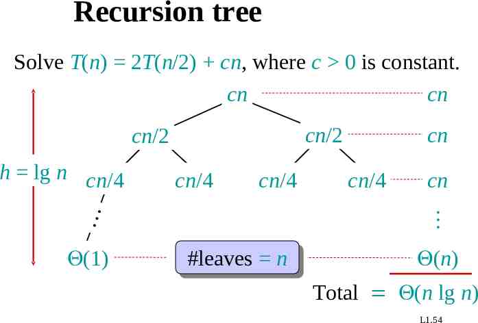
Recursion tree Solve T(n) 2T(n/2) cn, where c 0 is constant. L1.44
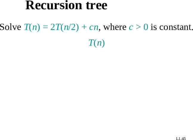
Recursion tree Solve T(n) 2T(n/2) cn, where c 0 is constant. T(n) L1.45
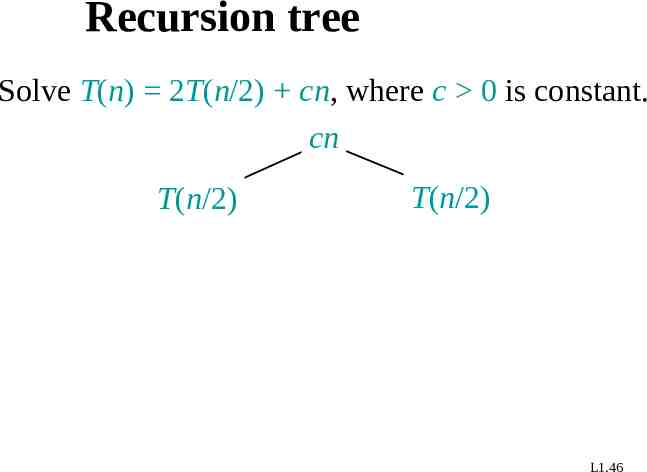
Recursion tree Solve T(n) 2T(n/2) cn, where c 0 is constant. cn T(n/2) T(n/2) L1.46
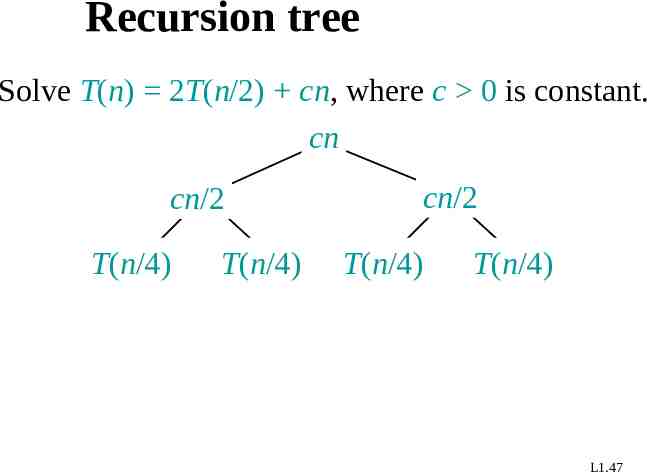
Recursion tree Solve T(n) 2T(n/2) cn, where c 0 is constant. cn cn/2 cn/2 T(n/4) T(n/4) T(n/4) T(n/4) L1.47
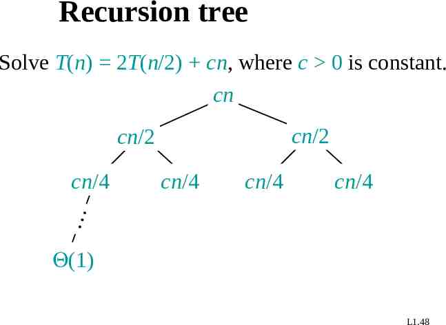
Recursion tree Solve T(n) 2T(n/2) cn, where c 0 is constant. cn cn/2 cn/2 cn/4 cn/4 cn/4 cn/4 (1) L1.48
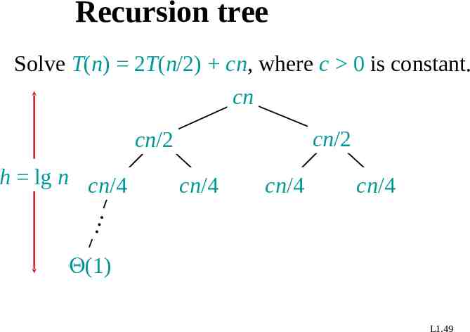
Recursion tree Solve T(n) 2T(n/2) cn, where c 0 is constant. cn cn/2 cn/2 cn/4 cn/4 cn/4 h lg n cn/4 (1) L1.49
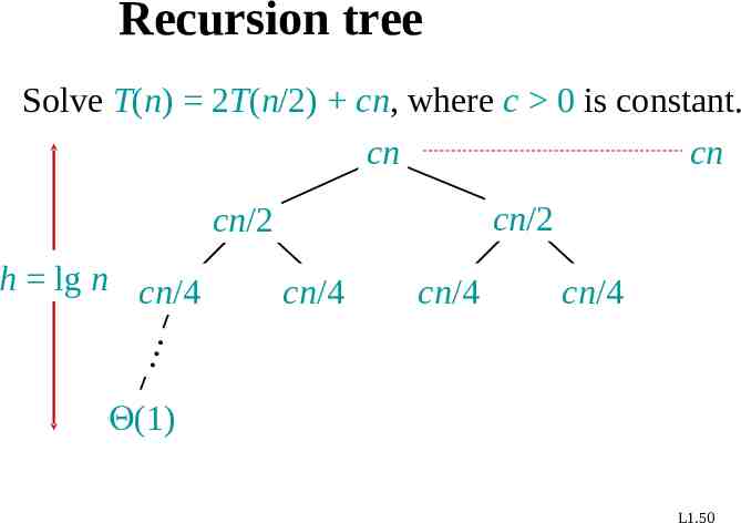
Recursion tree Solve T(n) 2T(n/2) cn, where c 0 is constant. cn cn cn/2 cn/2 cn/4 cn/4 cn/4 h lg n cn/4 (1) L1.50
Recursion tree Solve T(n) 2T(n/2) cn, where c 0 is constant. cn cn cn/2 cn/2 cn/4 cn/4 cn/4 h lg n cn/4 cn (1) L1.51
Recursion tree Solve T(n) 2T(n/2) cn, where c 0 is constant. cn cn h lg n cn/4 cn/4 cn/4 cn cn/4 cn cn/2 cn/2 (1) L1.52
Recursion tree Solve T(n) 2T(n/2) cn, where c 0 is constant. cn cn cn/2 cn/2 cn/4 cn/4 (1) cn/4 cn h lg n cn/4 cn #leaves n (n) L1.53
Recursion tree Solve T(n) 2T(n/2) cn, where c 0 is constant. cn cn cn/2 cn/2 cn/4 cn/4 (1) cn/4 cn h lg n cn/4 cn #leaves n (n) Total (n lg n) L1.54
Conclusions (n lg n) grows more slowly than (n2). Therefore, merge sort asymptotically beats insertion sort in the worst case. In practice, merge sort beats insertion sort for n 30 or so. L1.55