Hierarchical Tag visualization and application for tag recommendations


49 Slides2.99 MB
Hierarchical Tag visualization and application for tag recommendations CIKM’11 Advisor : Jia Ling, Koh Speaker : SHENG HONG, CHUNG 1
Outline Introduction Approach – Global tag ranking Information-theoretic tag ranking Learning-to-rank based tag ranking – Constructing tag hierarchy Tree initialization Iterative tag insertion Optimal position selection Applications to tag recommendation Experiment 2
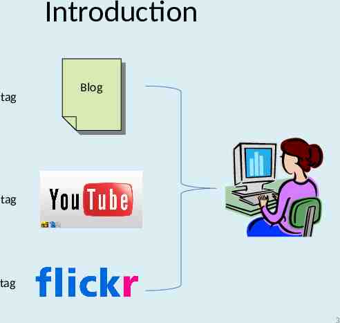
Introduction tag Blog Blog tag tag 3
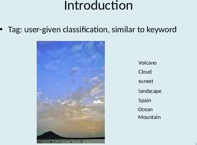
Introduction Tag: user-given classification, similar to keyword Volcano Cloud sunset landscape Spain Ocean Mountain 4
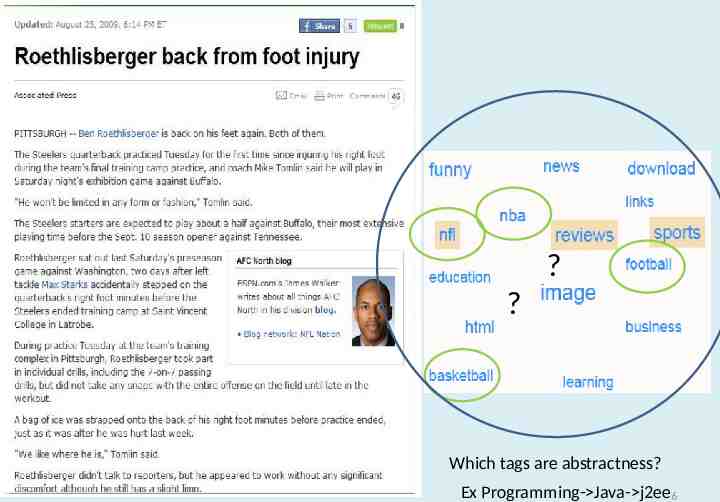
Introduction Tag visualization – Tag cloud Tag cloud Cloud Cloud landscape landscape Spain Spain Volcano sunset Ocean Mountain Mountain 5
? ? Which tags are abstractness? Ex Programming- Java- j2ee6
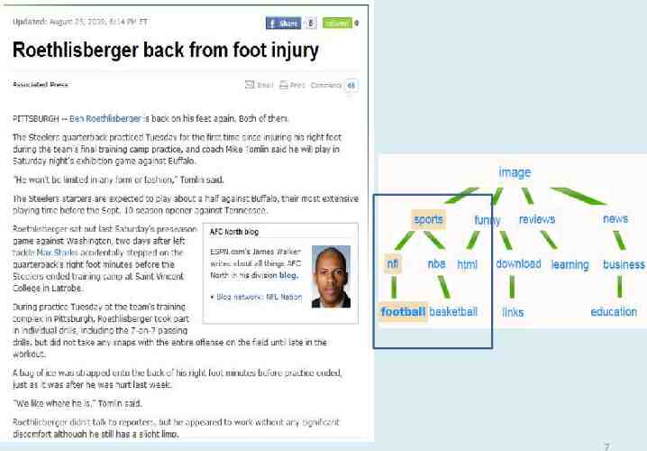
7
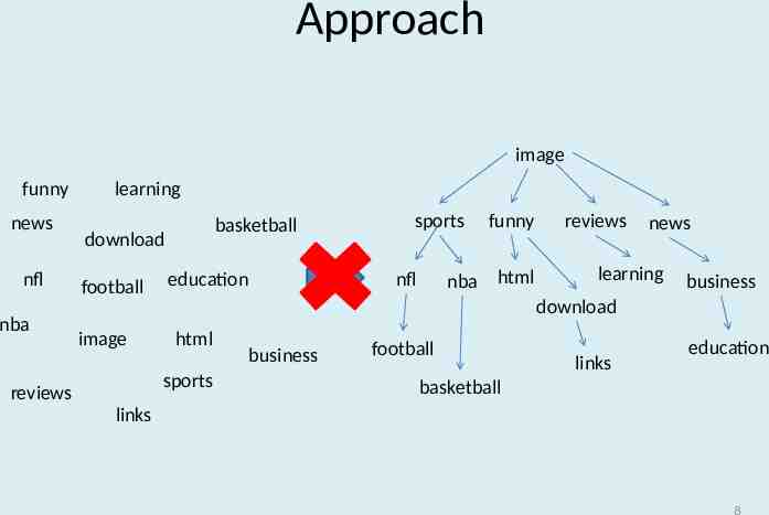
Approach image funny news nfl nba learning basketball download football image funny nba html nfl education reviews news learning business download html sports reviews sports business football links education basketball links 8
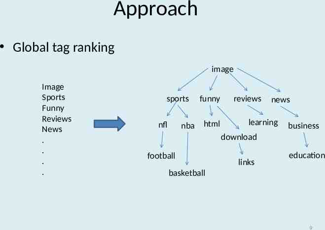
Approach Global tag ranking image Image Sports Funny Reviews News . . . . sports funny nba html nfl reviews news learning business download football links education basketball 9
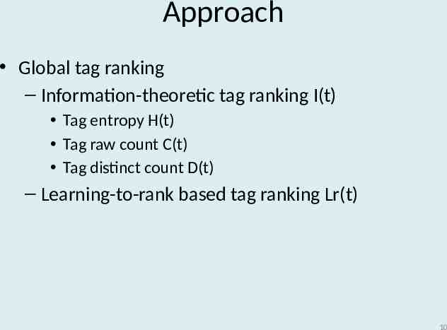
Approach Global tag ranking – Information-theoretic tag ranking I(t) Tag entropy H(t) Tag raw count C(t) Tag distinct count D(t) – Learning-to-rank based tag ranking Lr(t) 10
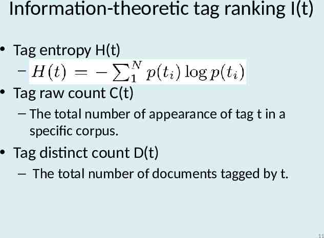
Information-theoretic tag ranking I(t) Tag entropy H(t) – Tag raw count C(t) – The total number of appearance of tag t in a specific corpus. Tag distinct count D(t) – The total number of documents tagged by t. 11
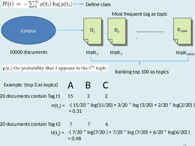
Define class Most frequent tag as topic Corpus DD1 1 DD2 2 10000 documents topic1 topic2 . . DD10000 10000 topic10000 Ranking top 100 as topics Example: (top 3 as topics) A B C 20 documents contain Tag t1 15 3 2 H(t1) -( 15/20 * log(15/20) 3/20 * log (3/20) 2/20 * log(2/20) ) 0.31 20 documents contain Tag t2 7 7 6 H(t2) -( 7/20 * log(7/20 ) 7/20 * log (7/20) 6/20 * log(6/20) ) 0.48 12
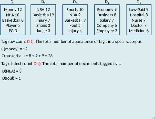
D1 D2 D3 D4 D5 Money 12 NBA 10 Basketball 8 Player 5 PG 3 NBA 12 Basketball 9 Injury 7 Shoes 3 Judge 3 Sports 10 NBA 9 Basketball 9 Foul 5 Injury 4 Economy 9 Business 8 Salary 7 Company 6 Employee 2 Low-Paid 9 Hospital 8 Nurse 7 Doctor 7 Medicine 6 Tag raw count C(t): The total number of appearance of tag t in a specific corpus. C(money) 12 C(basketball) 8 9 9 26 Tag distinct count D(t): The total number of documents tagged by t. D(NBA) 3 D(foul) 1 13
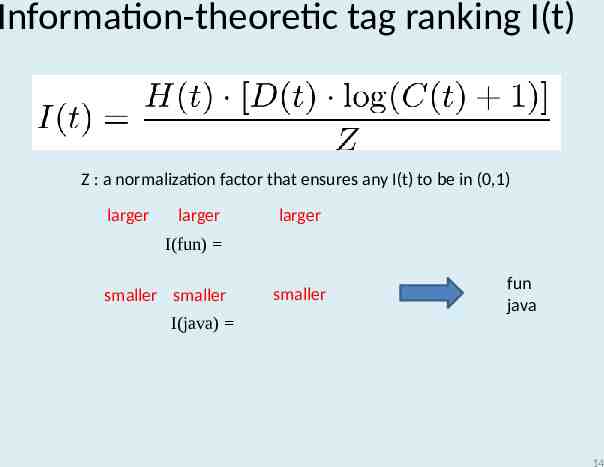
Information-theoretic tag ranking I(t) Z : a normalization factor that ensures any I(t) to be in (0,1) larger larger larger I(fun) smaller smaller I(java) smaller fun java 14
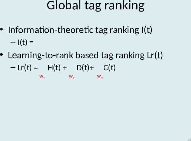
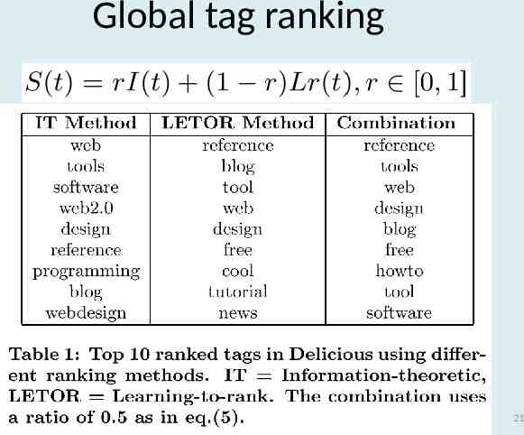
Global tag ranking Information-theoretic tag ranking I(t) – I(t) Learning-to-rank based tag ranking Lr(t) – Lr(t) H(t) w1 D(t) w2 C(t) w3 15
Learning-to-rank based tag ranking traingingdata? Time-consuming automatically generate 16
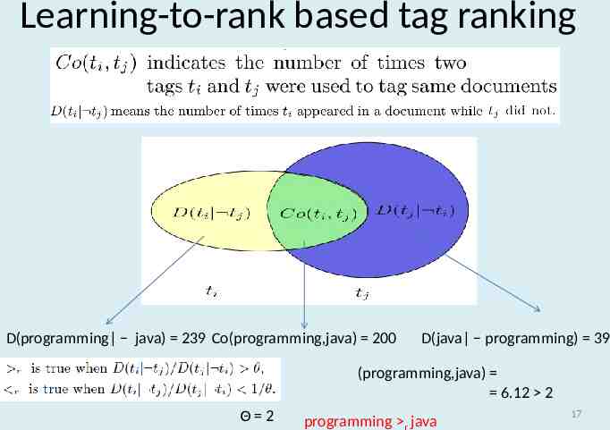
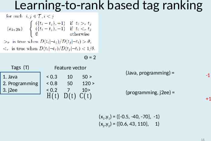
Learning-to-rank based tag ranking D(programming java) 239 Co(programming,java) 200 D(java programming) 39 (programming,java) 6.12 2 Θ 2 programming r java 17
Learning-to-rank based tag ranking Θ 2 Tags (T) 1. Java 2. Programming 3. j2ee Feature vector 0.3 0.8 0.2 10 50 7 50 120 10 H ( t ) D ( t ) C( t ) (Java, programming) -1 (programming, j2ee) 1 (x1,y1) ({-0.5, -40, -70}, -1) (x2,y2) ({0.6, 43, 110}, 1) 18
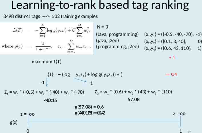
Learning-to-rank based tag ranking 3498 distinct tags --- 532 training examples N 3 (Java, programming) (java, j2ee) (programming, j2ee) (x1,y1) ({-0.5, -40, -70}, -1) (x2,y2) ({0.1, 3, 40}, 0) (x3,y3) ({0.6, 43, 110}, 1) 1 maximum L(T) L(T) (log g( y1 z1 ) log g( y3 z3 )) ( -1 0.4 1 Z3 w1 * (0.6) w2 * (43) w3 * (110) 57.08 g(57.08) 0.6 g(-40.15) 0.4 g(40.15) 0.2 z oo Z1 w1 * (-0.5) w2 * (-40) w3 * (-70) 40.15 -40.15 z -oo g(z) 0 1 19
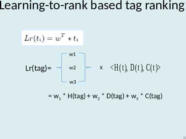
Learning-to-rank based tag ranking w1 Lr(tag) w2 X H(t), D(t ), C(t) w3 w1 * H(tag) w2 * D(tag) w3 * C(tag) 20
Global tag ranking 21
Constructing tag hierarchy Goal – select appropriate tags to be included in the tree – choose the optimal position for those tags Steps – Tree initialization – Iterative tag insertion – Optimal position selection 22
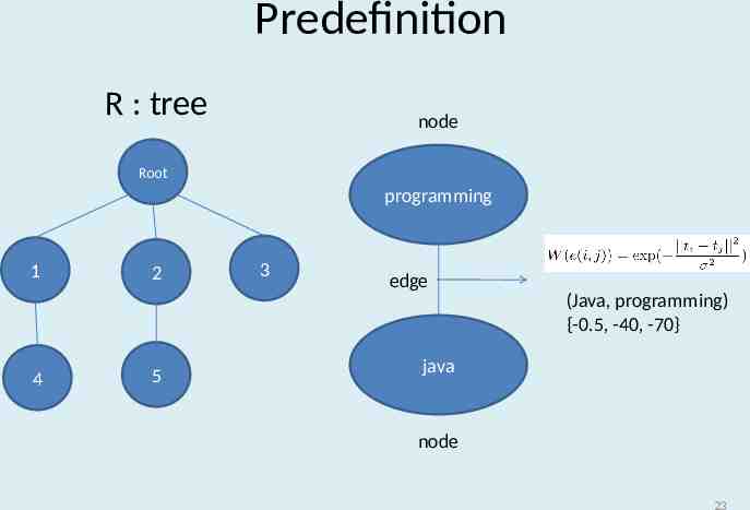
Predefinition R : tree node Root programming 1 2 3 edge (Java, programming) {-0.5, -40, -70} 4 5 java node 23
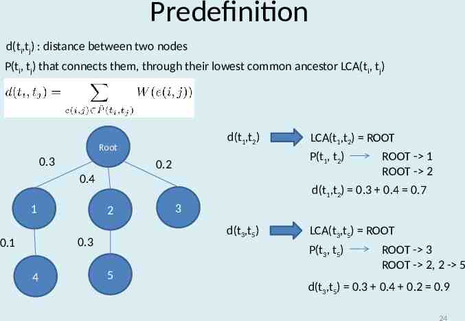
Predefinition d(ti,tj) : distance between two nodes P(ti, tj) that connects them, through their lowest common ancestor LCA(ti, tj) d(t1,t2) Root 0.3 P(t1, t2) 0.2 0.4 1 4 ROOT - 1 ROOT - 2 d(t1,t2) 0.3 0.4 0.7 2 3 d(t3,t5) 0.3 0.1 LCA(t1,t2) ROOT LCA(t3,t5) ROOT P(t3, t5) 5 ROOT - 3 ROOT - 2, 2 - 5 d(t3,t5) 0.3 0.4 0.2 0.9 24
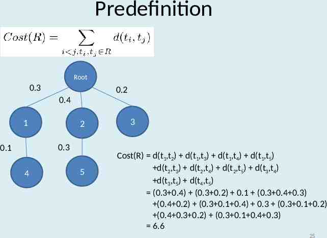
Predefinition Root 0.3 0.2 0.4 1 2 0.3 0.1 4 5 3 Cost(R) d(t1,t2) d(t1,t3) d(t1,t4) d(t1,t5) d(t2,t3) d(t2,t4) d(t2,t5) d(t3,t4) d(t3,t5) d(t4,t5) (0.3 0.4) (0.3 0.2) 0.1 (0.3 0.4 0.3) (0.4 0.2) (0.3 0.1 0.4) 0.3 (0.3 0.1 0.2) (0.4 0.3 0.2) (0.3 0.1 0.4 0.3) 6.6 25
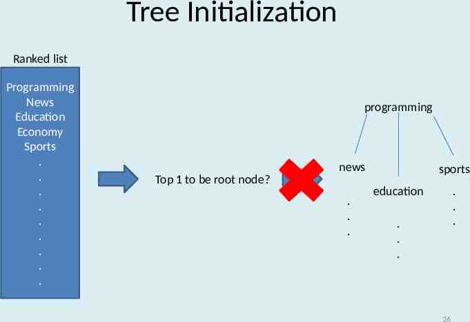
Tree Initialization Ranked list Programming News Education Economy Sports . . . . . . . . . programming news Top 1 to be root node? . . . sports education . . . . . . 26
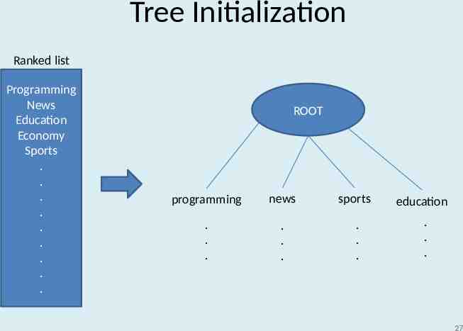
Tree Initialization Ranked list Programming News Education Economy Sports . . . . . . . . . ROOT programming news sports . . . . . . . . . education . . . 27
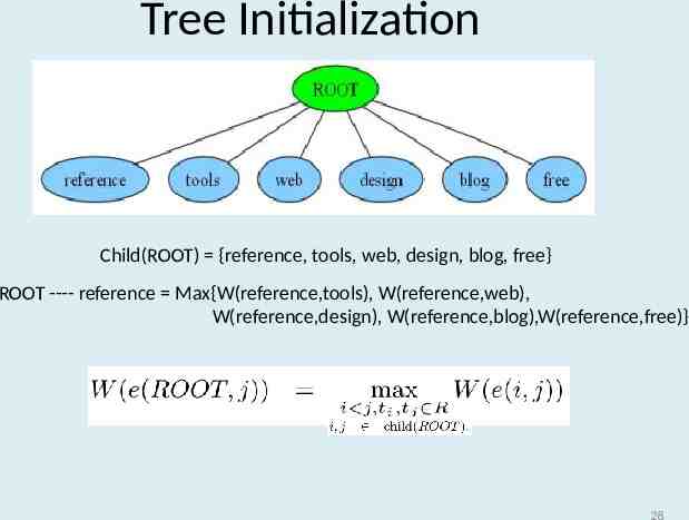
Tree Initialization Child(ROOT) {reference, tools, web, design, blog, free} ROOT ---- reference Max{W(reference,tools), W(reference,web), W(reference,design), W(reference,blog),W(reference,free)} 28
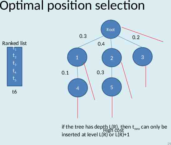
Optimal position selection Root 0.3 Ranked list t1 t2 t3 t4 t5 t6 0.2 0.4 1 2 3 0.3 0.1 4 5 if the tree has depth L(R), then tnew can only be High cost inserted at level L(R) or L(R) 1 29
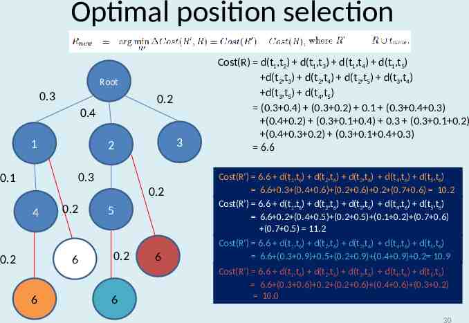
Optimal position selection Root 0.3 0.2 0.4 1 3 2 0.3 0.1 0.2 4 0.2 0.2 6 6 5 0.2 6 6 Cost(R) d(t1,t2) d(t1,t3) d(t1,t4) d(t1,t5) d(t2,t3) d(t2,t4) d(t2,t5) d(t3,t4) d(t3,t5) d(t4,t5) (0.3 0.4) (0.3 0.2) 0.1 (0.3 0.4 0.3) (0.4 0.2) (0.3 0.1 0.4) 0.3 (0.3 0.1 0.2) (0.4 0.3 0.2) (0.3 0.1 0.4 0.3) 6.6 Cost(R’) 6.6 d(t1,t6) d(t2,t6) d(t3,t6) d(t4,t6) d(t5,t6) 6.6 0.3 (0.4 0.6) (0.2 0.6) 0.2 (0.7 0.6) 10.2 Cost(R’) 6.6 d(t1,t6) d(t2,t6) d(t3,t6) d(t4,t6) d(t5,t6) 6.6 0.2 (0.4 0.5) (0.2 0.5) (0.1 0.2) (0.7 0.6) (0.7 0.5) 11.2 Cost(R’) 6.6 d(t1,t6) d(t2,t6) d(t3,t6) d(t4,t6) d(t5,t6) 6.6 (0.3 0.9) 0.5 (0.2 0.9) (0.4 0.9) 0.2 10.9 Cost(R’) 6.6 d(t1,t6) d(t2,t6) d(t3,t6) d(t4,t6) d(t5,t6) 6.6 (0.3 0.6) 0.2 (0.2 0.6) (0.4 0.6) (0.3 0.2) 10.0 30
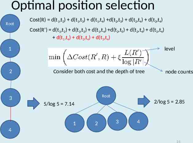
Optimal position selection Root Cost(R) d(t1,t2) d(t1,t3) d(t1,t4) d(t2,t3) d(t2,t4) d(t3,t4) Cost(R’) d(t1,t2) d(t1,t3) d(t1,t4) d(t2,t3) d(t2,t4) d(t3,t4) d(t1,t4) d(t2,t4) d(t3,t4) level 1 2 Consider both cost and the depth of tree node counts Root 3 2/log 5 2.85 5/log 5 7.14 1 2 3 4 4 31
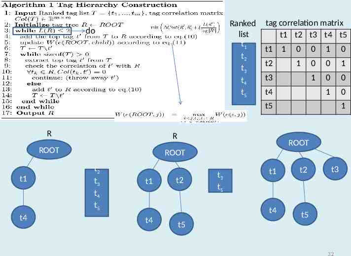
Ranked list t1 t2 t3 t4 t5 do tag correlation matrix t1 t2 t3 t4 t5 t1 t2 1 0 0 1 0 1 0 0 1 1 0 0 1 0 t3 t4 t5 R R ROOT t1 t4 1 ROOT ROOT t2 t3 t4 t5 t1 t2 t3 t5 t1 t4 t4 t2 t3 t5 t5 32
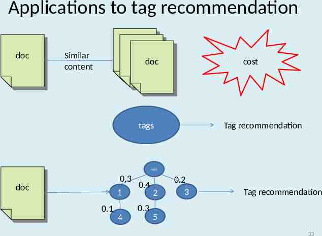
Applications to tag recommendation doc doc Similar content cost doc doc Tag recommendation tags root 0.3 doc doc 1 0.1 0.4 0.3 4 2 0.2 3 Tag recommendation 5 33
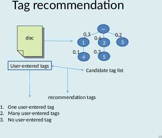
Tag recommendation root 0.3 doc doc 1 0.1 User-entered tags 0.4 0.3 4 2 0.2 3 5 Candidate tag list recommendation tags 1. One user-entered tag 2. Many user-entered tags 3. No user-entered tag 34
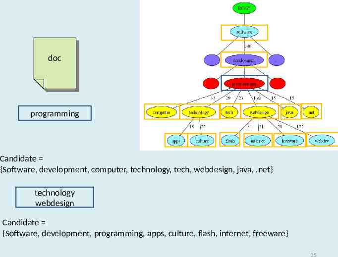
doc doc programming Candidate {Software, development, computer, technology, tech, webdesign, java, .net} technology webdesign Candidate {Software, development, programming, apps, culture, flash, internet, freeware} 35
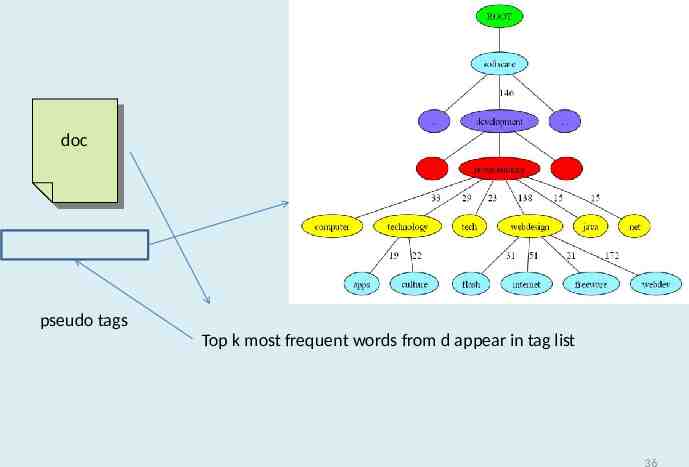
doc doc pseudo tags Top k most frequent words from d appear in tag list 36
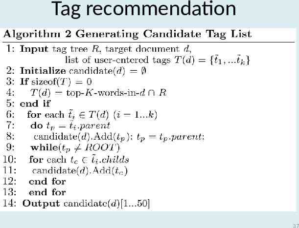
Tag recommendation 37
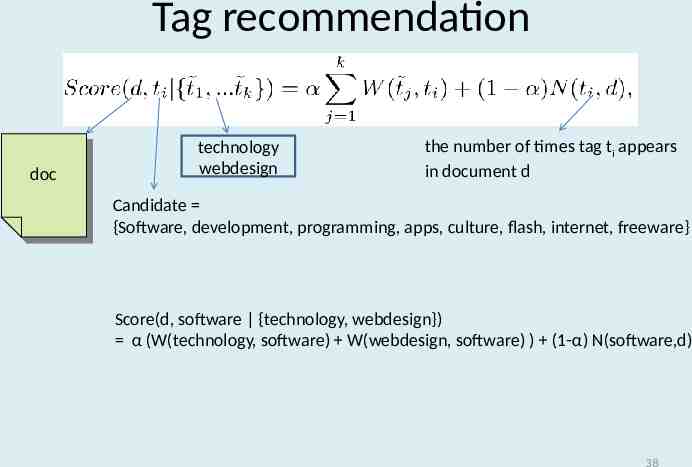
Tag recommendation doc doc technology webdesign the number of times tag ti appears in document d Candidate {Software, development, programming, apps, culture, flash, internet, freeware} Score(d, software {technology, webdesign}) α (W(technology, software) W(webdesign, software) ) (1-α) N(software,d) 38
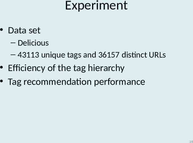
Experiment Data set – Delicious – 43113 unique tags and 36157 distinct URLs Efficiency of the tag hierarchy Tag recommendation performance 39
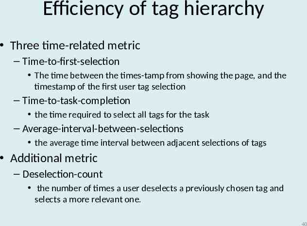
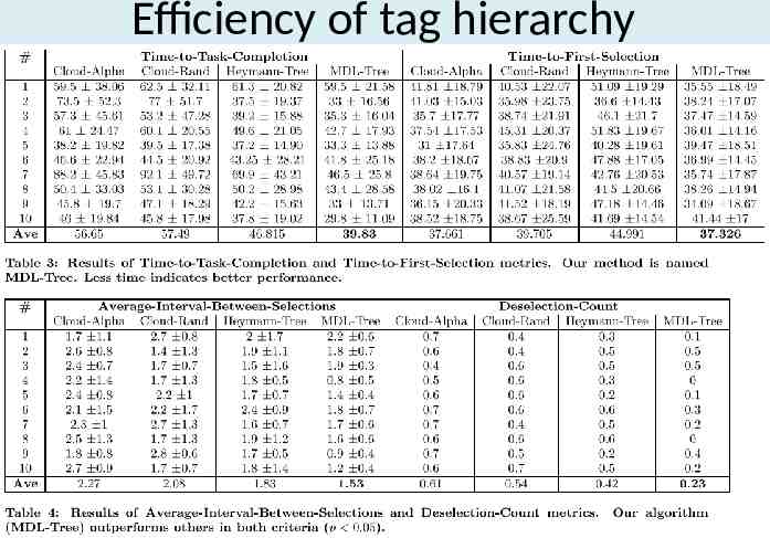
Efficiency of tag hierarchy Three time-related metric – Time-to-first-selection The time between the times-tamp from showing the page, and the timestamp of the first user tag selection – Time-to-task-completion the time required to select all tags for the task – Average-interval-between-selections the average time interval between adjacent selections of tags Additional metric – Deselection-count the number of times a user deselects a previously chosen tag and selects a more relevant one. 40
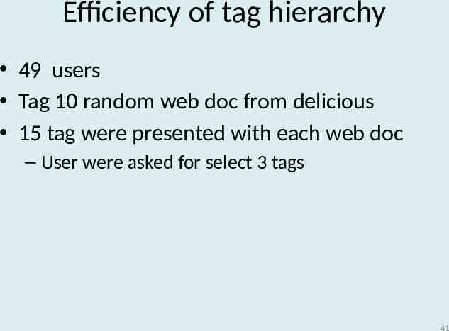
Efficiency of tag hierarchy 49 users Tag 10 random web doc from delicious 15 tag were presented with each web doc – User were asked for select 3 tags 41
42
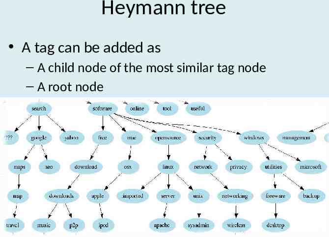
Heymann tree A tag can be added as – A child node of the most similar tag node – A root node 43
Efficiency of tag hierarchy 44
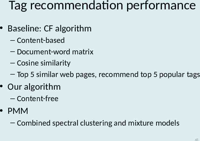
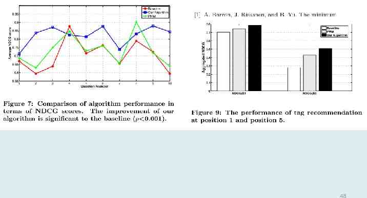
Tag recommendation performance Baseline: CF algorithm – Content-based – Document-word matrix – Cosine similarity – Top 5 similar web pages, recommend top 5 popular tags Our algorithm – Content-free PMM – Combined spectral clustering and mixture models 45
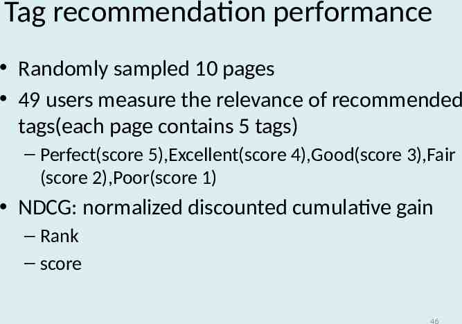
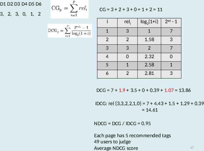
Tag recommendation performance Randomly sampled 10 pages 49 users measure the relevance of recommended tags(each page contains 5 tags) – Perfect(score 5),Excellent(score 4),Good(score 3),Fair (score 2),Poor(score 1) NDCG: normalized discounted cumulative gain – Rank – score 46
D1 D2 D3 D4 D5 D6 3, 2, 3, 0, 1, 2 CG 3 2 3 0 1 2 11 i reli log2(1 i) 2rel - 1 1 3 1 7 2 2 1.58 3 3 3 2 7 4 0 2.32 0 5 1 2.58 1 6 2 2.81 3 DCG 7 1.9 3.5 0 0.39 1.07 13.86 IDCG: rel {3,3,2,2,1,0} 7 4.43 1.5 1.29 0.39 14.61 NDCG DCG / IDCG 0.95 Each page has 5 recommended tags 49 users to judge Average NDCG score 47
48
Conclusion We proposed a novel visualization of tag hierarchy whic addresses two shortcomings of traditional tag clouds: – unable to capture the similarities between tags – unable to organize tags into levels of abstractness Our visualization method can reduce the tagging time Our tag recommendation algorithm outperformed a content-based recommendation method in NDCG score 49