Dense Matrix Algorithms Carl Tropper Department of Computer Science

58 Slides2.30 MB
Dense Matrix Algorithms Carl Tropper Department of Computer Science McGill University
Dense Few non-zero entries Topics – Matrix-Vector Multiplication – Matrix-Matrix Multiplication – Solving a System of Linear Equations
Introductory ramblings Due to their regular structure, parallel computations involving matrices and vectors readily lend themselves to datadecomposition. Typical algorithms rely on input, output, or intermediate data decomposition. Discuss one-and two-dimensional block, cyclic, and block-cyclic partitionings. Use one task per process
Matrix-Vector Multiplication Multiply a dense n x n matrix A with an n x 1 vector x to yield an n x 1 vector y. The serial algorithm requires n2 multiplications and additions.
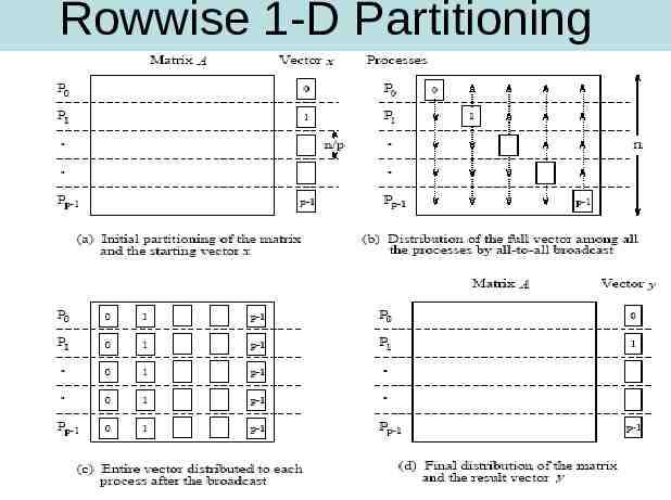
Rowwise 1-D Partitioning
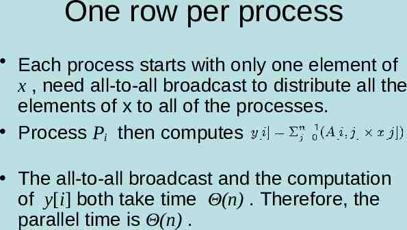
One row per process Each process starts with only one element of x , need all-to-all broadcast to distribute all the elements of x to all of the processes. Process Pi then computes The all-to-all broadcast and the computation of y[i] both take time Θ(n) . Therefore, the parallel time is Θ(n) .
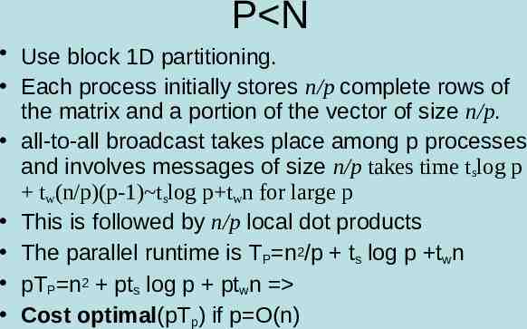
P N Use block 1D partitioning. Each process initially stores n/p complete rows of the matrix and a portion of the vector of size n/p. all-to-all broadcast takes place among p processes and involves messages of size n/p takes time tslog p tw(n/p)(p-1) tslog p twn for large p This is followed by n/p local dot products The parallel runtime is TP n2/p ts log p twn pTP n2 pts log p ptwn Cost optimal(pTp) if p O(n)
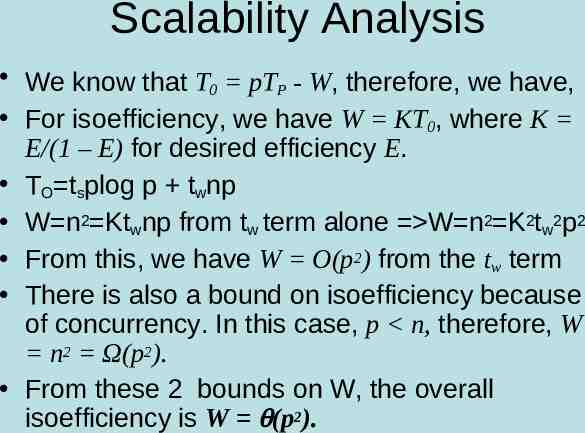
Scalability Analysis We know that T0 pTP - W, therefore, we have, For isoefficiency, we have W KT0, where K E/(1 – E) for desired efficiency E. TO tsplog p twnp W n2 Ktwnp from tw term alone W n2 K2tw2p2 From this, we have W O(p2) from the tw term There is also a bound on isoefficiency because of concurrency. In this case, p n, therefore, W n2 Ω(p2). From these 2 bounds on W, the overall isoefficiency is W (p2).
2-D Partitioning (naïve version) Begin with one element per process partitioning The n x n matrix is partitioned among n2 processors such that each processor owns a single element. The n x 1 vector x is distributed in the last column of n processors.Each processor has one element.
2-D Partitioning
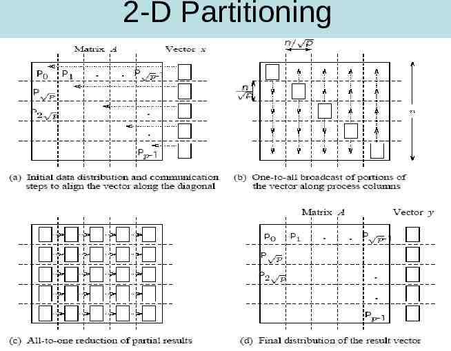
2-D Partitioning We must first align the vector with the matrix appropriately. The first communication step for the 2-D partitioning aligns the vector x along the principal diagonal of the matrix. The second step copies the vector elements from each diagonal process to all the processes in the corresponding column using n simultaneous broadcasts among all processors in the column. Finally, the result vector is computed by performing an all-to-one reduction along the columns.
2-D Partitioning Three basic communication operations are used in this algorithm: – one-to-one communication to align the vector along the main diagonal, – one-to-all broadcast of each vector element among the n processes of each column, and – all-to-one reduction in each row. Each of these operations takes Θ(log n) time and the parallel time is Θ(log n) . There are n2 processes,so the cost (process-time product) is Θ(n2 log n) ; hence, the algorithm is not cost-optimal.
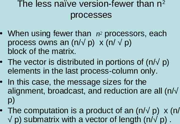
The less naïve version-fewer than n2 processes When using fewer than n2 processors, each process owns an (n/ p) x (n/ p) block of the matrix. The vector is distributed in portions of (n/ p) elements in the last process-column only. In this case, the message sizes for the alignment, broadcast, and reduction are all (n/ p) The computation is a product of an (n/ p) x (n/ p) submatrix with a vector of length (n/ p) .
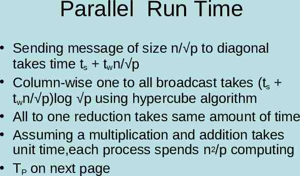
Parallel Run Time Sending message of size n/ p to diagonal takes time ts twn/ p Column-wise one to all broadcast takes (ts twn/ p)log p using hypercube algorithm All to one reduction takes same amount of time Assuming a multiplication and addition takes unit time,each process spends n2/p computing TP on next page
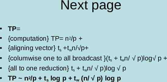
Next page TP {computation} TP n2/p {aligning vector} ts twn/ p {columwise one to all broadcast }(ts twn/ p)log p {all to one reduction} ts twn/ p)log p TP n2/p ts log p tw (n/ p) log p
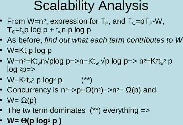
Scalability Analysis From W n2, expression for TP, and TO pTP-W, TO tsp log p twn p log p As before, find out what each term contributes to W W Ktsp log p W n2 Ktwn plog p n Ktw p log p n2 K2tw2 p log 2p W K2tw2 p log2 p (**) Concurrency is n2 p O(n2) n2 Ω(p) and W Ω(p) The tw term dominates (**) everything W (p log2 p )
Scalability Analysis Maximum number of processes which can be used cost-optimally for a problem of size W is determined by p log2 p O(n2) After some manipulation, p O(n2/log2n), Asymptotic upper bound on the number of processes which can be used for cost-otpimal solution Bottom line:2-D partitioning is better than 1-D because: It is faster! It has a smaller isoefficiency function-get the same efficiency on more processes!
Matrix-Matrix multiplication Standard serial algorithm involves taking the dot product of each row with each column, has complexity of n3 Can also use q x q array of blocks, where each block is (n/q x n/q). This yields q3 multiplications and additions of the submatrices. Each of the sub-matrices involves (n/q)3 additions and multiplications. Paralellize the q x q blocks algorithm.
Simple Parallel Algorithm A and B are partitioned into p blocks, i.e. AIJ , BIJ of size (n/ p x n/ p) They are mapped onto a p x p mesh PI,J stores AI,J and BI,J and computes CI,J Needs AI,K and BJ,K sub-matrices 0 k p All to all broadcast of A’s blocks done on each row and of B’s blocks on each column Then multiply A’s and B’s
Scalability 2 all to all broadcasts of process mesh Messages contain submatrices of n2/p elements Communication time is 2(ts log ( p) tw (n2/p)( p-1) {hypercube is assumed} Each process computes C I,J-takes p multiplications (n/ p x n/ p) submatrices, taking n3/p time. Parallel time TP n3/p ts log p 2 tw n2/ p Process time product n3 tsplog p 2twn2 p Cost optimal for p O(n2)
Scalability The isoefficiency is O(p1.5) due to bandwidth term tw and concurrency Major drawback-algorithm is not memory optimal-Memory is (n2 p), or p times the memory of the sequential algorithm
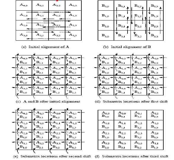
Canon’s algorithm Idea: schedule the computations of the processes of the ith row such that at any given time each process uses a different block Ai,k. These blocks can be systematically rotated among the processes after every submatrix multiplication so that every process gets a fresh Ai,k after each rotation Use same algorithm for columns no process holds more then one bock at a time Memory is (n2)
Canon shift
Performance Max shift for a block is p-1. 2 shifts (row and column) require 2(ts twn2/p) P shifts p2(ts twn2/p) total comm time The time for multiplying p matrices of size (n/ p) x (n/ p) is n3/p TP n3/p p2(ts twn2/p) Same cost-optimality condition as simple algorithm and same iso function. Difference is memory!!
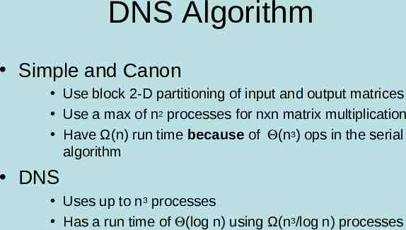
DNS Algorithm Simple and Canon Use block 2-D partitioning of input and output matrices Use a max of n2 processes for nxn matrix multiplication Have Ω(n) run time because of (n3) ops in the serial algorithm DNS Uses up to n3 processes Has a run time of (log n) using Ω(n3/log n) processes
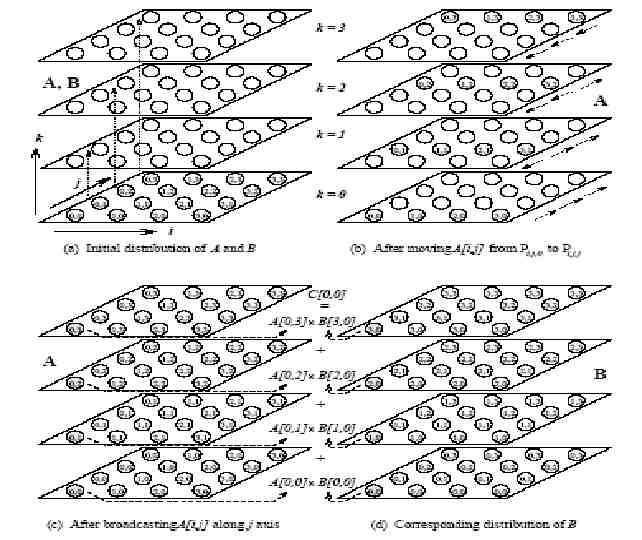
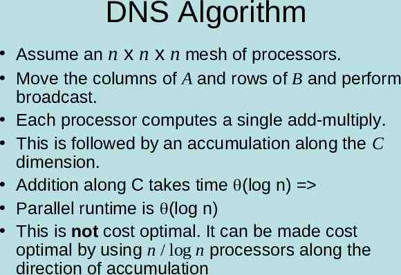
DNS Algorithm Assume an n x n x n mesh of processors. Move the columns of A and rows of B and perform broadcast. Each processor computes a single add-multiply. This is followed by an accumulation along the C dimension. Addition along C takes time (log n) Parallel runtime is (log n) This is not cost optimal. It can be made cost optimal by using n / log n processors along the direction of accumulation
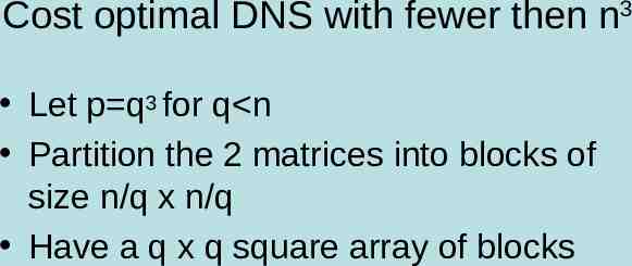
Cost optimal DNS with fewer then n3 Let p q3 for q n Partition the 2 matrices into blocks of size n/q x n/q Have a q x q square array of blocks
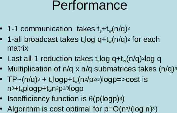
Performance 1-1 communication takes ts tw(n/q)2 1-all broadcast takes tslog q tw(n/q)2 for each matrix Last all-1 reduction takes tslog q tw(n/q)2log q Multiplication of n/q x n/q submatrices takes (n/q)3 TP (n/q)3 tslogp tw(n2/p2/3)logp cost is n3 tsplogp twn2p1/3logp Isoefficiency function is (p(logp)3) Algorithm is cost optimal for p O(n3/(log n)3)
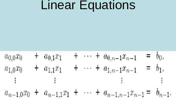
Linear Equations
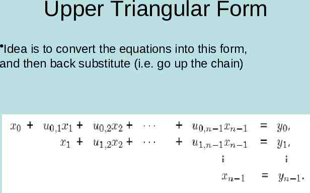
Upper Triangular Form Idea is to convert the equations into this form, and then back substitute (i.e. go up the chain)
Principle behind solution Can make use of elementary operations on equations to solve them Elementary operations are Interchanging two rows Replace any equation by a linear combination of any other equation and itself
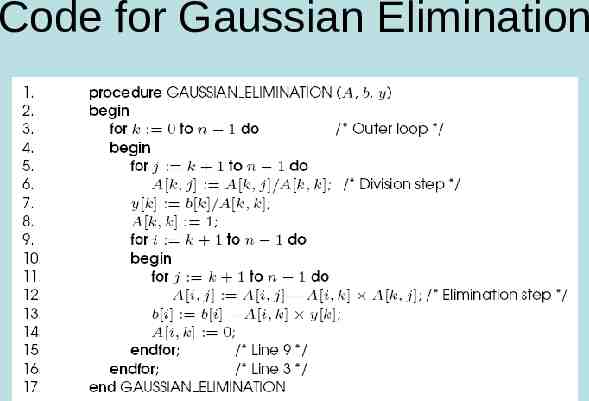
Code for Gaussian Elimination
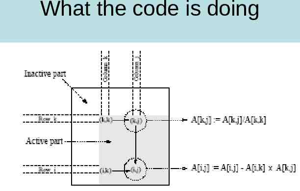
What the code is doing
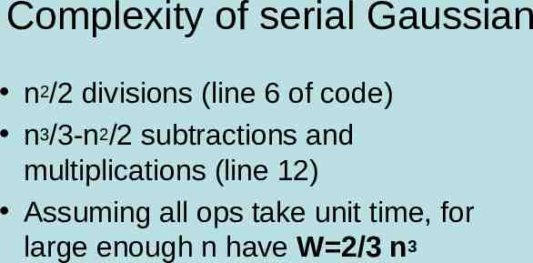
Complexity of serial Gaussian n2/2 divisions (line 6 of code) n3/3-n2/2 subtractions and multiplications (line 12) Assuming all ops take unit time, for large enough n have W 2/3 n3
Parallel Gaussian Use 1-D Partitioning One row per process
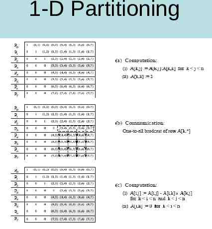
1-D Partitioning
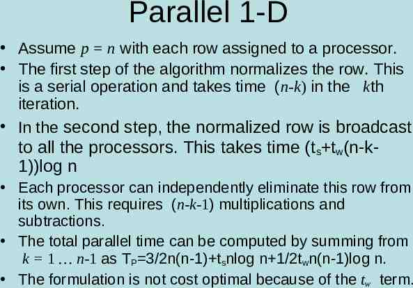
Parallel 1-D Assume p n with each row assigned to a processor. The first step of the algorithm normalizes the row. This is a serial operation and takes time (n-k) in the kth iteration. In the second step, the normalized row is broadcast to all the processors. This takes time (t s tw(n-k1))log n Each processor can independently eliminate this row from its own. This requires (n-k-1) multiplications and subtractions. The total parallel time can be computed by summing from k 1 n-1 as TP 3/2n(n-1) tsnlog n 1/2twn(n-1)log n. The formulation is not cost optimal because of the tw term.
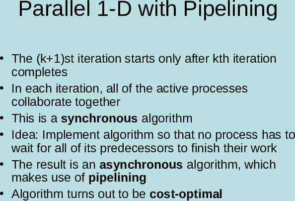
Parallel 1-D with Pipelining The (k 1)st iteration starts only after kth iteration completes In each iteration, all of the active processes collaborate together This is a synchronous algorithm Idea: Implement algorithm so that no process has to wait for all of its predecessors to finish their work The result is an asynchronous algorithm, which makes use of pipelining Algorithm turns out to be cost-optimal
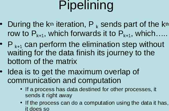
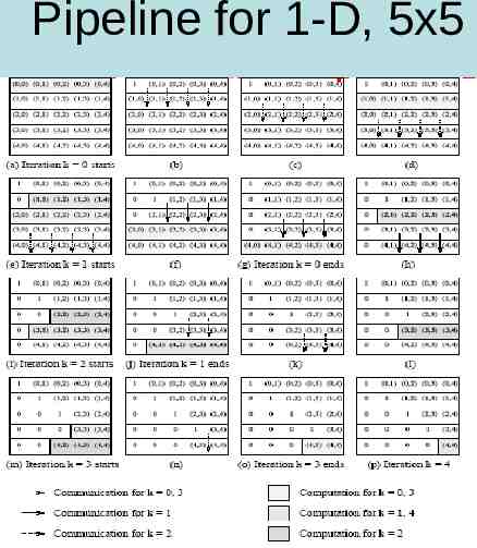
Pipelining During the kth iteration, P k sends part of the kth row to Pk 1, which forwards it to Pk 1, which . P k 1 can perform the elimination step without waiting for the data finish its journey to the bottom of the matrix Idea is to get the maximum overlap of communication and computation If a process has data destined for other processes, it sends it right away If the process can do a computation using the data it has, it does so
Pipeline for 1-D, 5x5
Pipelining is cost optimal The total number of steps in the entire pipelined procedure is Θ(n). In any step, either O(n) elements are communicated between directly-connected processes, or a division step is performed on O(n) elements of a row, or an elimination step is performed on O(n) elements of a row. The parallel time is therefore O(n2) Since there are n processes, the cost is O(n3) Guess what,cost optimal!
Pipelining 1-D with p n Pipelining algorithm can be easily extended N x N matrix n/p processes per processor Example on next slide P 4 8 x8 matrix
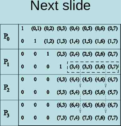
Next slide
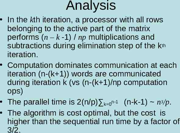
Analysis In the kth iteration, a processor with all rows belonging to the active part of the matrix performs (n – k -1) / np multiplications and subtractions during elimination step of the kth iteration. Computation dominates communication at each iteration (n-(k 1)) words are communicated during iteration k (vs (n-(k 1)/np computation ops) The parallel time is 2(n/p) k 0n-1 (n-k-1) n3/p. The algorithm is cost optimal, but the cost is higher than the sequential run time by a factor of 3/2.
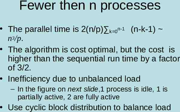
Fewer then n processes The parallel time is 2(n/p) k 0n-1 (n-k-1) n3/p. The algorithm is cost optimal, but the cost is higher than the sequential run time by a factor of 3/2. Inefficiency due to unbalanced load – In the figure on next slide,1 process is idle, 1 is partially active, 2 are fully active Use cyclic block distribution to balance load
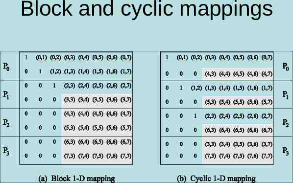
Block and cyclic mappings
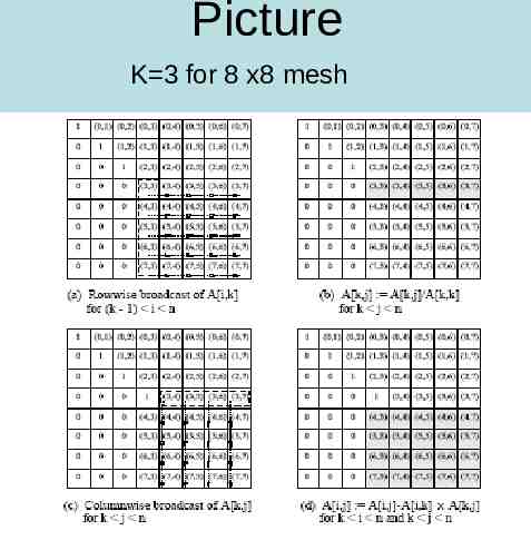
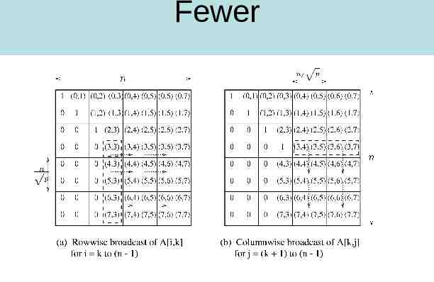
2-D Partitioning A[i,j] is n x n and is mapped to n x n mesh-A[i,j] goes to P I,J The rest is as before, only the communication of individual elements takes place between processors Need one to all broadcast of A[i,k] along ith row for k i n and one to all broadcast of A[k,j] along jth column for k j n Picture on next slide The result is not cost optimal
Picture K 3 for 8 x8 mesh
Pipeline If we use synchronous broadcasts, the results are not cost optimal, so we pipeline the 2-D algorithm Principle of the pipelining algorithm is the same-if you can compute or communicate, do it now, not later – P k,k 1 can divide A[k,k 1] by A[k,k] before A[k,k 1] reaches P k,n-1 {the end of the row} – After A[k,j] performs the division, it can send the result down column j without waiting Next slide exhibits algorithm for 2-D pipelining
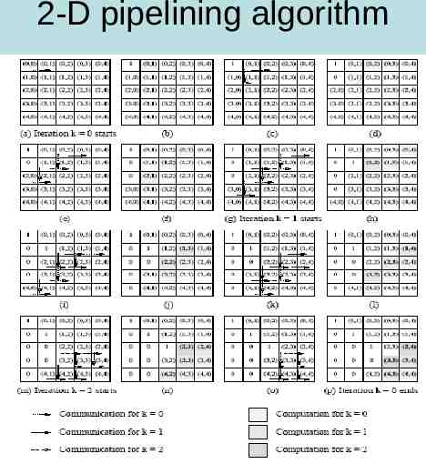
2-D pipelining algorithm
Pipelining-the wave The computation and communication for each iteration moves through the mesh from top-left to bottom-right like a wave After the wave corresponding to a certain iteration passes through a process, the process is free to perform subsequent iterations. In g, after k 0 wave passes P 1,1 it starts k 1 iteration by passing A[1,1] to P 1,2. Multiple wave that correspond to different iterations are active simultaneously.
The wave-continued If each step (division, elimination, or communication) is assumed to take constant time, the front moves a single step in this time. The front takes Θ(n) time to reach Pn-1,n-1. Once the front has progressed past a diagonal processor, the next front can be initiated. In this way, the last front passes the bottom-right corner of the matrix Θ(n) steps after the first one. The parallel time is therefore O(n) , which is cost-optimal.
Fewer then n proceses 2 In this case, a processor containing an active part of the matrix performs n2/p multiplications and subtractions, and communicates n/ p words along its row and its column. The computation dominates communication for n p. The total parallel run time of this algorithm is (2n2/p) x n, since there are n iterations. Process time product 2n3/p x p 2n3 This is three times the serial operation count!
Fewer
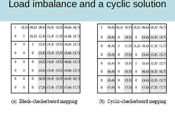
Load imbalance Same problem as with 1-D mapping-an uneven load distribution Same solution-cyclic partitioning
Load imbalance and a cyclic solution
Comparison Pipelined version takes (n3/p) time on p processes for both 1-D and 2-D versions 2-D partitioning can use more processes O(n2) then 1-D partitioning O(n) for an n x n matrix 2-D version is more scalable