SOLVING LINEAR PROGRAMMING PROBLEMS: The Simplex Method

63 Slides662.50 KB
SOLVING LINEAR PROGRAMMING PROBLEMS: The Simplex Method
Simplex Method Used for solving LP problems will be presented Put into the form of a table, and then a number of mathematical steps are performed on the table Moves from one extreme point on the solution boundary to another until the best one is found, and then it stops A lengthy and tedious process but computer software programs are now used easily instead Programs do not provide an in-depth understanding of how those solutions are derived Can greatly enhance one's understanding of LP
First Step First step is to convert model into standard form s1 and s2, represent amount of unused labor and wood No chairs and tables are produced, s1 40 and s2 120 Unused resources contribute nothing to profit, Z 0 Decision variables as well as profit at origin are:
Assigning (n-m) Variables Equal to Zero Determine values of variables at every possible solution point Have two equations and four unknowns, which makes direct simultaneous solution impossible Assigns n-m variables 0 – n number of variables – m number of constraints Have n 4 variables and m 2 constraints x1 0 and s1 0 and substituting them results in x2 20 and s2 60
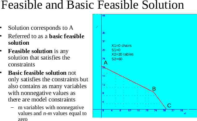
Feasible and Basic Feasible Solution Solution corresponds to A Referred to as a basic feasible solution Feasible solution is any solution that satisfies the constraints Basic feasible solution not only satisfies the constraints but also contains as many variables with nonnegative values as there are model constraints – m variables with nonnegative values and n-m values equal to zero A X1 0 chairs S1 0 X2 20 tables S2 60 B C
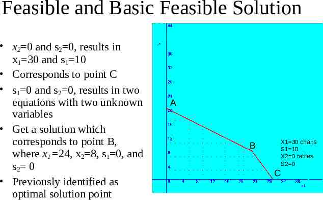
Feasible and Basic Feasible Solution x2 0 and s2 0, results in x1 30 and s1 10 Corresponds to point C s1 0 and s2 0, results in two equations with two unknown variables Get a solution which corresponds to point B, where x1 24, x2 8, s1 0, and s2 0 Previously identified as optimal solution point A B X1 30 chairs S1 10 X2 0 tables S2 0 C
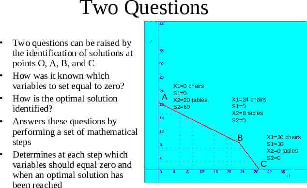
Two Questions Two questions can be raised by the identification of solutions at points O, A, B, and C How was it known which variables to set equal to zero? How is the optimal solution identified? Answers these questions by performing a set of mathematical steps Determines at each step which variables should equal zero and when an optimal solution has been reached A X1 0 chairs S1 0 X2 20 tables S2 60 X1 24 chairs S1 0 X2 8 tables S2 0 B X1 30 chairs S1 10 X2 0 tables S2 0 C
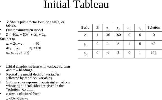
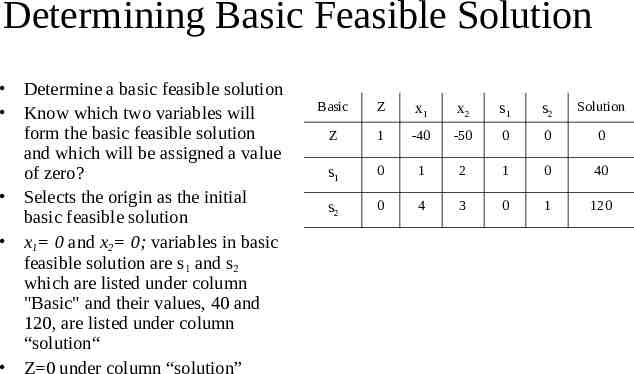
Initial Tableau Model is put into the form of a table, or tableau Our maximization model Z 40x1 50x2 0s1 0s2 Subject to x1 2x2 s1 40 4x1 3x2 s2 120 x1, x2 , s1, s2 0 Initial simplex tableau with various column and row headings Record the model decision variables, followed by the slack variables Bottom rows represent constraint equations whose right-hand sides are given in the “solution” column z-row is obtained from z -40x1-50x2 0 Basic Z x1 x2 s1 s2 Solution Z 1 -40 -50 0 0 0 s1 0 1 2 1 0 40 s2 0 4 3 0 1 120
Determining Basic Feasible Solution Determine a basic feasible solution Know which two variables will form the basic feasible solution and which will be assigned a value of zero? Selects the origin as the initial basic feasible solution x1 0 and x2 0; variables in basic feasible solution are s1 and s2 which are listed under column "Basic" and their values, 40 and 120, are listed under column “solution“ Z 0 under column “solution” Basic Z x1 x2 s1 s2 Solution Z 1 -40 -50 0 0 0 s1 0 1 2 1 0 40 s2 0 4 3 0 1 120
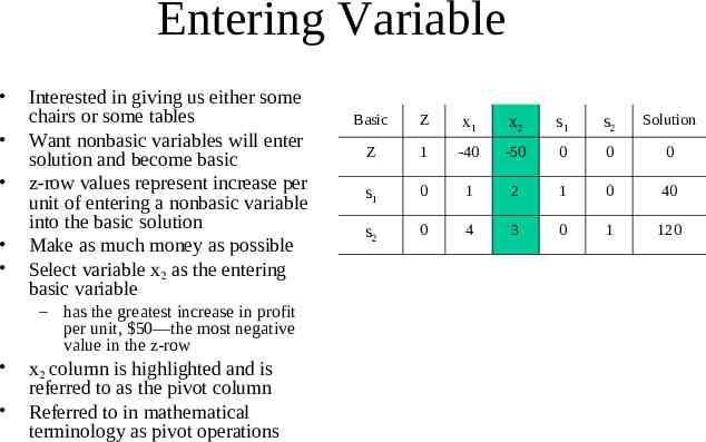
Entering Variable Interested in giving us either some chairs or some tables Want nonbasic variables will enter solution and become basic z-row values represent increase per unit of entering a nonbasic variable into the basic solution Make as much money as possible Select variable x2 as the entering basic variable – has the greatest increase in profit per unit, 50—the most negative value in the z-row x2 column is highlighted and is referred to as the pivot column Referred to in mathematical terminology as pivot operations Basic Z x1 x2 s1 s2 Solution Z 1 -40 -50 0 0 0 s1 0 1 2 1 0 40 s2 0 4 3 0 1 120
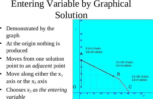
Entering Variable by Graphical Solution Demonstrated by the graph At the origin nothing is produced Moves from one solution point to an adjacent point Move along either the x1 axis or the x2 axis Chooses x2 as the entering variable A X1 0 chairs X2 20 tables X1 24 chairs X2 8 tables B O X1 30 chairs X2 0 tables C
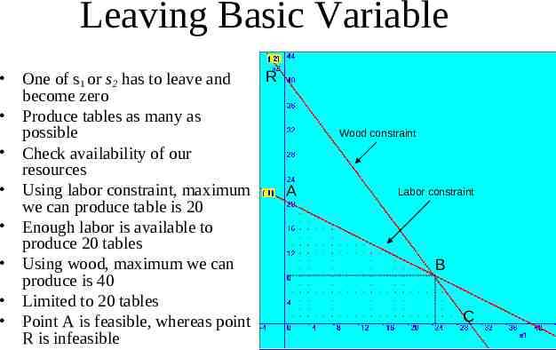
Leaving Basic Variable R One of s1 or s2 has to leave and become zero Produce tables as many as possible Check availability of our resources Using labor constraint, maximum A we can produce table is 20 Enough labor is available to produce 20 tables Using wood, maximum we can produce is 40 Limited to 20 tables Point A is feasible, whereas point R is infeasible Wood constraint Labor constraint B C
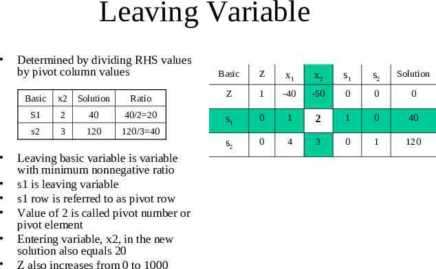
Leaving Variable Determined by dividing RHS values by pivot column values Basic x2 Solution Ratio S1 2 40 40/2 20 s2 3 120 120/3 40 Leaving basic variable is variable with minimum nonnegative ratio s1 is leaving variable s1 row is referred to as pivot row Value of 2 is called pivot number or pivot element Entering variable, x2, in the new solution also equals 20 Z also increases from 0 to 1000 Basic Z x1 x2 s1 s2 Solution Z 1 -40 -50 0 0 0 s1 0 1 2 1 0 40 s2 0 4 3 0 1 120
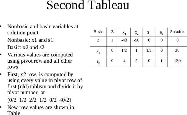
Second Tableau Nonbasic and basic variables at solution point Nonbasic: x1 and s1 Basic: x2 and s2 Various values are computed using pivot row and all other rows First, x2 row, is computed by using every value in pivot row of first (old) tableau and divide it by pivot number, or (0/2 1/2 2/2 1/2 0/2 40/2) New row values are shown in Table Basic Z x1 x2 s1 s2 Solution Z 1 -40 -50 0 0 0 x2 0 1/2 1 1/2 0 20 s2 0 4 3 0 1 120
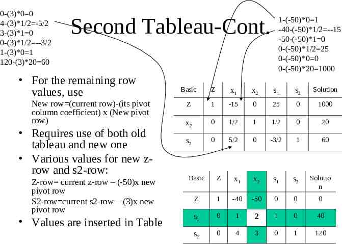
0-(3)*0 0 4-(3)*1/2 -5/2 3-(3)*1 0 0-(3)*1/2 --3/2 1-(3)*0 1 120-(3)*20 60 Second Tableau-Cont. For the remaining row values, use New row (current row)-(its pivot column coefficient) x (New pivot row) Requires use of both old tableau and new one Various values for new zrow and s2-row: Z-row current z-row – (-50)x new pivot row S2-row current s2-row – (3)x new pivot row Values are inserted in Table 1-(-50)*0 1 -40-(-50)*1/2 --15 -50-(-50)*1 0 0-(-50)*1/2 25 0-(-50)*0 0 0-(-50)*20 1000 Basic Z x1 x2 s1 s2 Solution Z 1 -15 0 25 0 1000 x2 0 1/2 1 1/2 0 20 s2 0 5/2 0 -3/2 1 60 Basic Z x1 x2 s1 s2 Solutio n Z 1 -40 -50 0 0 0 s1 0 1 2 1 0 40 s2 0 4 3 0 1 120
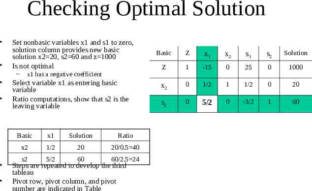
Checking Optimal Solution Set nonbasic variables x1 and s1 to zero, solution column provides new basic solution x2 20, s2 60 and z 1000 Is not optimal – x1 has a negative coefficient Select variable x1 as entering basic variable Ratio computations, show that s2 is the leaving variable Basic x1 Solution Ratio x2 1/2 20 20/0.5 40 s2 5/2 60 60/2.5 24 Steps are repeated to develop the third tableau Pivot row, pivot column, and pivot number are indicated in Table Basic Z x1 x2 s1 s2 Solution Z 1 -15 0 25 0 1000 x2 0 1/2 1 1/2 0 20 s2 0 5/2 0 -3/2 1 60
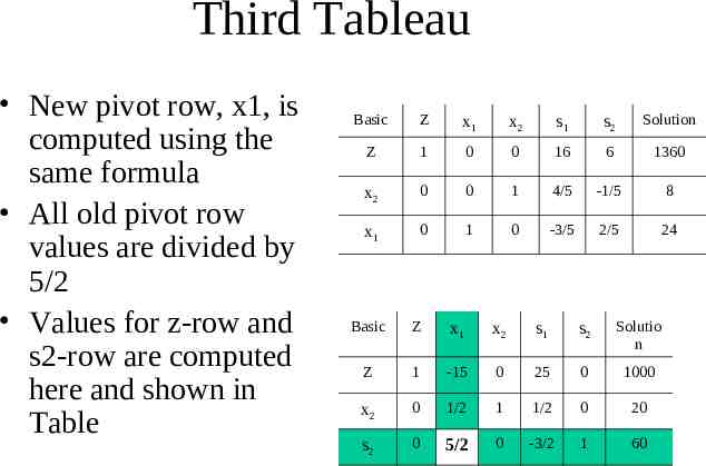
Third Tableau New pivot row, x1, is computed using the same formula All old pivot row values are divided by 5/2 Values for z-row and s2-row are computed here and shown in Table Basic Z x1 x2 s1 s2 Solution Z 1 0 0 16 6 1360 x2 0 0 1 4/5 -1/5 8 x1 0 1 0 -3/5 2/5 24 Basic Z x1 x2 s1 s2 Solutio n Z 1 -15 0 25 0 1000 x2 0 1/2 1 1/2 0 20 s2 0 5/2 0 -3/2 1 60
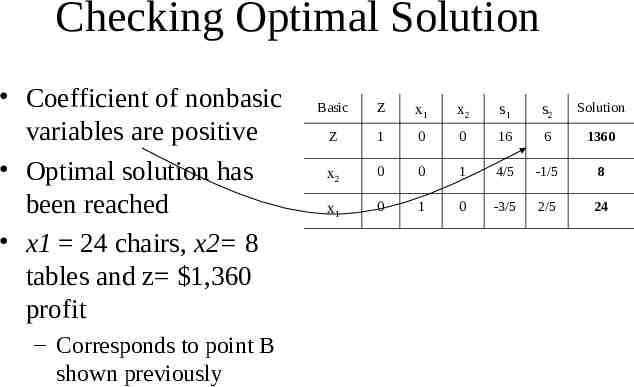
Checking Optimal Solution Coefficient of nonbasic variables are positive Optimal solution has been reached x1 24 chairs, x2 8 tables and z 1,360 profit – Corresponds to point B shown previously Basic Z x1 x2 s1 s2 Solution Z 1 0 0 16 6 1360 x2 0 0 1 4/5 -1/5 8 x1 0 1 0 -3/5 2/5 24
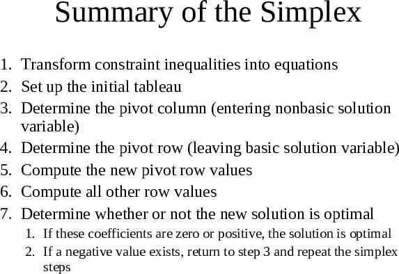
Summary of the Simplex 1. Transform constraint inequalities into equations 2. Set up the initial tableau 3. Determine the pivot column (entering nonbasic solution variable) 4. Determine the pivot row (leaving basic solution variable) 5. Compute the new pivot row values 6. Compute all other row values 7. Determine whether or not the new solution is optimal 1. If these coefficients are zero or positive, the solution is optimal 2. If a negative value exists, return to step 3 and repeat the simplex steps
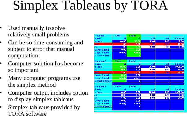
Simplex Tableaus by TORA Used manually to solve relatively small problems Can be so time-consuming and subject to error that manual computation Computer solution has become so important Many computer programs use the simplex method Computer output includes option to display simplex tableaus Simplex tableaus provided by TORA software
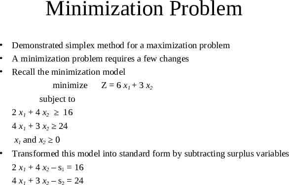
Minimization Problem Demonstrated simplex method for a maximization problem A minimization problem requires a few changes Recall the minimization model minimize Z 6 x1 3 x2 subject to 2 x1 4 x2 16 4 x1 3 x2 24 x1 and x2 0 Transformed this model into standard form by subtracting surplus variables 2 x1 4 x2 – s1 16 4 x1 3 x2 – s2 24
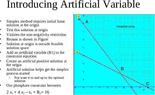
Introducing Artificial Variable Simplex method requires initial basic solution at the origin Test this solution at origin Violates the non-negativity restriction Reason is shown in Figure Solution at origin is outside feasible solution space Add an artificial variable (R1) to the constraint equation Create an artificial positive solution at the origin Artificial solution helps get the simplex process started – Not want it to end up in the optimal solution Our phosphate constraint becomes 2 x1 4 x2 – s1 R1 16 A Feasible area B C
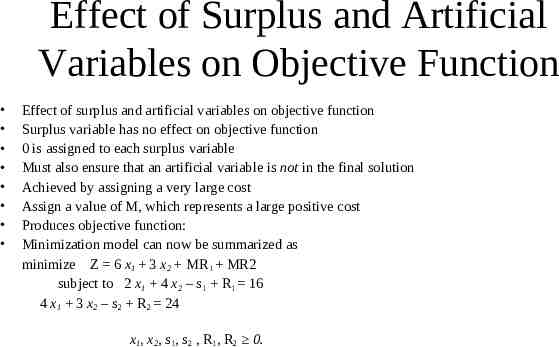
Effect of Surplus and Artificial Variables on Objective Function Effect of surplus and artificial variables on objective function Surplus variable has no effect on objective function 0 is assigned to each surplus variable Must also ensure that an artificial variable is not in the final solution Achieved by assigning a very large cost Assign a value of M, which represents a large positive cost Produces objective function: Minimization model can now be summarized as minimize Z 6 x1 3 x2 MR1 MR2 subject to 2 x1 4 x2 – s1 R1 16 4 x1 3 x2 – s2 R2 24 x1, x2, s1, s2 , R1, R2 0.
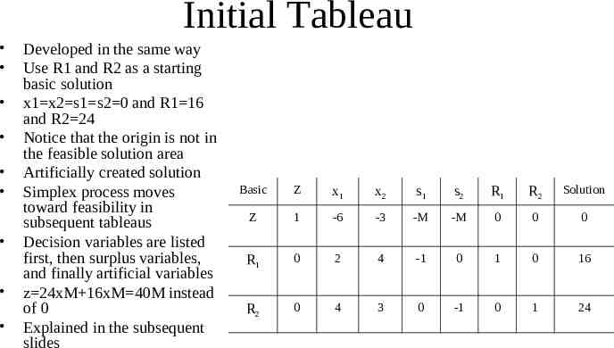
Initial Tableau Developed in the same way Use R1 and R2 as a starting basic solution x1 x2 s1 s2 0 and R1 16 and R2 24 Notice that the origin is not in the feasible solution area Artificially created solution Simplex process moves toward feasibility in subsequent tableaus Decision variables are listed first, then surplus variables, and finally artificial variables z 24xM 16xM 40M instead of 0 Explained in the subsequent slides Basic Z x1 x2 s1 s2 R1 R2 Solution Z 1 -6 -3 -M -M 0 0 0 R1 0 2 4 -1 0 1 0 16 R2 0 4 3 0 -1 0 1 24
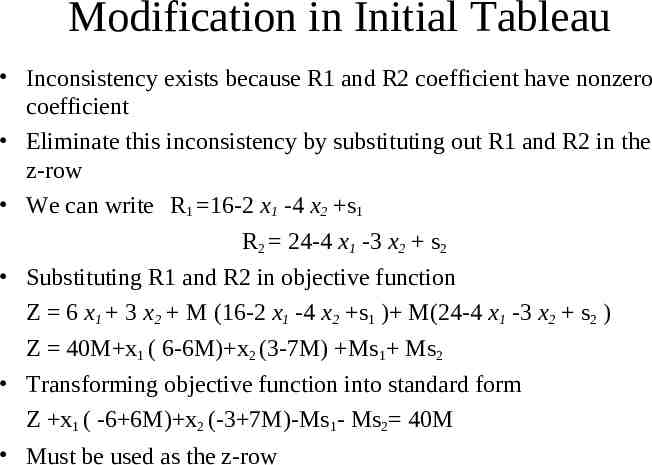
Modification in Initial Tableau Inconsistency exists because R1 and R2 coefficient have nonzero coefficient Eliminate this inconsistency by substituting out R1 and R2 in the z-row We can write R1 16-2 x1 -4 x2 s1 R2 24-4 x1 -3 x2 s2 Substituting R1 and R2 in objective function Z 6 x1 3 x2 M (16-2 x1 -4 x2 s1 ) M(24-4 x1 -3 x2 s2 ) Z 40M x1 ( 6-6M) x2 (3-7M) Ms1 Ms2 Transforming objective function into standard form Z x1 ( -6 6M) x2 (-3 7M)-Ms1- Ms2 40M Must be used as the z-row
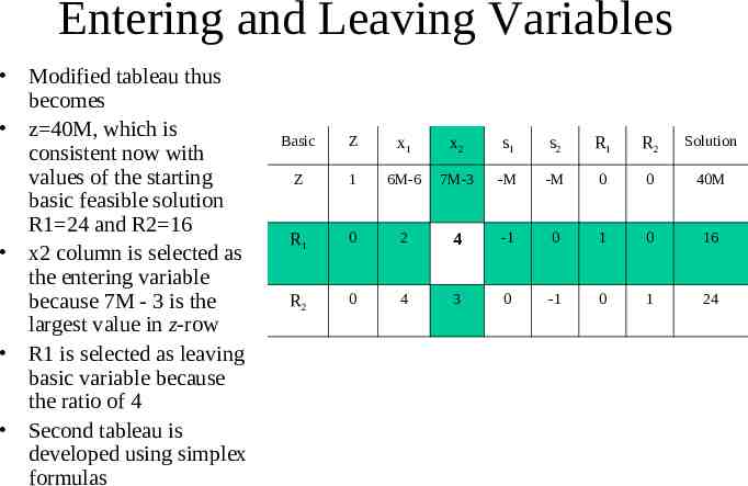
Entering and Leaving Variables Modified tableau thus becomes z 40M, which is consistent now with values of the starting basic feasible solution R1 24 and R2 16 x2 column is selected as the entering variable because 7M - 3 is the largest value in z-row R1 is selected as leaving basic variable because the ratio of 4 Second tableau is developed using simplex formulas Basic Z x1 x2 s1 s2 R1 R2 Solution Z 1 6M-6 7M-3 -M -M 0 0 40M R1 0 2 4 -1 0 1 0 16 R2 0 4 3 0 -1 0 1 24
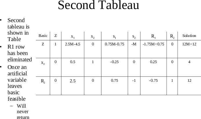
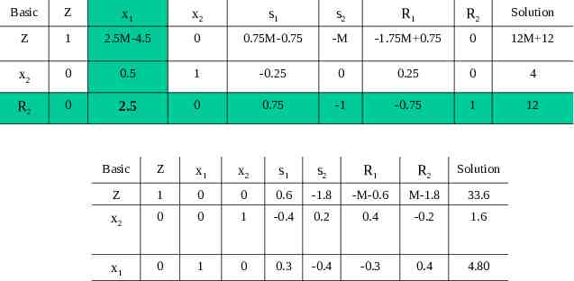
Second Tableau Second tableau is shown in Table R1 row has been eliminated Once an artificial variable leaves basic feasible – Will never return Basic Z x1 x2 s1 s2 R1 R2 Solution Z 1 2.5M-4.5 0 0.75M-0.75 -M -1.75M 0.75 0 12M 12 x2 0 0.5 1 -0.25 0 0.25 0 4 R2 0 2.5 0 0.75 -1 -0.75 1 12
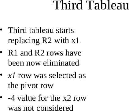
Third Tableau Third tableau starts replacing R2 with x1 R1 and R2 rows have been now eliminated x1 row was selected as the pivot row -4 value for the x2 row was not considered
Basic Z x1 x2 s1 s2 R1 R2 Solution Z 1 2.5M-4.5 0 0.75M-0.75 -M -1.75M 0.75 0 12M 12 x2 0 0.5 1 -0.25 0 0.25 0 4 R2 0 2.5 0 0.75 -1 -0.75 1 12 Basic Z x1 x2 s1 s2 R1 R2 Solution Z 1 0 0 0.6 -1.8 -M-0.6 M-1.8 33.6 x2 0 0 1 -0.4 0.2 0.4 -0.2 1.6 x1 0 1 0 0.3 -0.4 -0.3 0.4 4.80
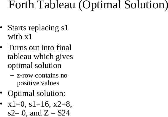
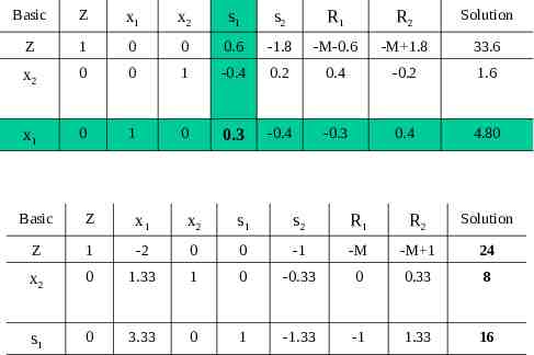
Forth Tableau (Optimal Solution) Starts replacing s1 with x1 Turns out into final tableau which gives optimal solution – z-row contains no positive values Optimal solution: x1 0, s1 16, x2 8, s2 0, and Z 24
Basic Z x1 x2 s1 s2 R1 R2 Solution Z 1 0 0 0.6 -1.8 -M-0.6 -M 1.8 33.6 x2 0 0 1 -0.4 0.2 0.4 -0.2 1.6 x1 0 1 0 0.3 -0.4 -0.3 0.4 4.80 Basic Z x1 x2 s1 s2 R1 R2 Solution Z 1 -2 0 0 -1 -M -M 1 24 x2 0 1.33 1 0 -0.33 0 0.33 8 s1 0 3.33 0 1 -1.33 -1 1.33 16
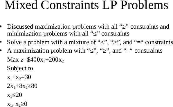
Mixed Constraints LP Problems Discussed maximization problems with all “ ” constraints and minimization problems with all “ ” constraints Solve a problem with a mixture of “ ”, “ ”, and “ “ constraints A maximization problem with “ ”, “ ”, and “ “ constraints Max z 400x1 200x2 Subject to x1 x2 30 2x1 8x2 80 x1 20 x1, x2 0
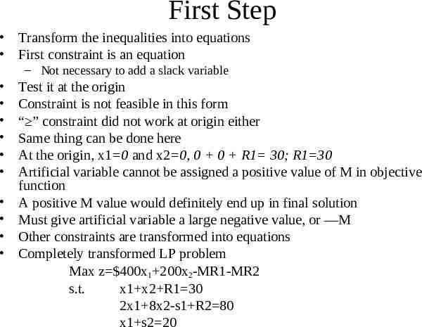
First Step Transform the inequalities into equations First constraint is an equation – Not necessary to add a slack variable Test it at the origin Constraint is not feasible in this form “ ” constraint did not work at origin either Same thing can be done here At the origin, x1 0 and x2 0, 0 0 R1 30; R1 30 Artificial variable cannot be assigned a positive value of M in objective function A positive M value would definitely end up in final solution Must give artificial variable a large negative value, or —M Other constraints are transformed into equations Completely transformed LP problem Max z 400x1 200x2-MR1-MR2 s.t. x1 x2 R1 30 2x1 8x2-s1 R2 80 x1 s2 20
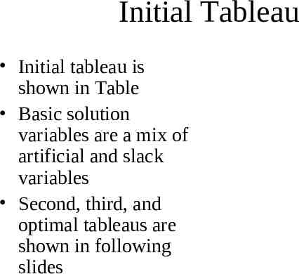
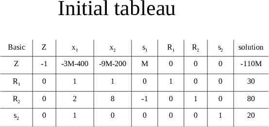
Initial Tableau Initial tableau is shown in Table Basic solution variables are a mix of artificial and slack variables Second, third, and optimal tableaus are shown in following slides
Initial tableau Basic Z x1 x2 s1 R1 R2 s2 solution Z -1 -3M-400 -9M-200 M 0 0 0 -110M R1 0 1 1 0 1 0 0 30 R2 0 2 8 -1 0 1 0 80 s2 0 1 0 0 0 0 1 20
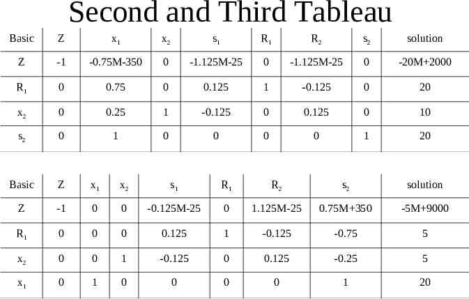
Second and Third Tableau Basic Z x1 x2 s1 R1 R2 s2 solution Z -1 -0.75M-350 0 -1.125M-25 0 -1.125M-25 0 -20M 2000 R1 0 0.75 0 0.125 1 -0.125 0 20 x2 0 0.25 1 -0.125 0 0.125 0 10 s2 0 1 0 0 0 0 1 20 Basic Z x1 x2 s1 R1 R2 s2 solution Z -1 0 0 -0.125M-25 0 1.125M-25 0.75M 350 -5M 9000 R1 0 0 0 0.125 1 -0.125 -0.75 5 x2 0 0 1 -0.125 0 0.125 -0.25 5 x1 0 1 0 0 0 0 1 20
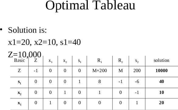
Optimal Tableau Solution is: x1 20, x2 10, s1 40 Z 10,000 Basic Z x1 x2 s1 R1 R2 s2 solution Z -1 0 0 0 M 200 M 200 10000 s1 0 0 0 1 8 -1 -6 40 x2 0 0 1 0 1 0 -1 10 x1 0 1 0 0 0 0 1 20
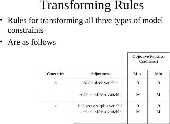
Transforming Rules Rules for transforming all three types of model constraints Are as follows Objective Function Coefficient Constraint Adjustment Max Min Add a slack variable 0 0 Add an artificial variable -M M Subtract a surplus variable add an artificial variable 0 -M 0 M
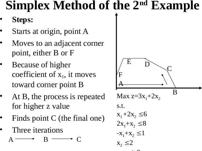
Simplex Method of the 2nd Example Steps: Starts at origin, point A Moves to an adjacent corner point, either B or F Because of higher coefficient of x1, it moves toward corner point B At B, the process is repeated for higher z value Finds point C (the final one) Three iterations A B C E D F A Max z 3x1 2x2 s.t. x1 2x2 6 2x1 x2 8 -x1 x2 1 x2 2 C B
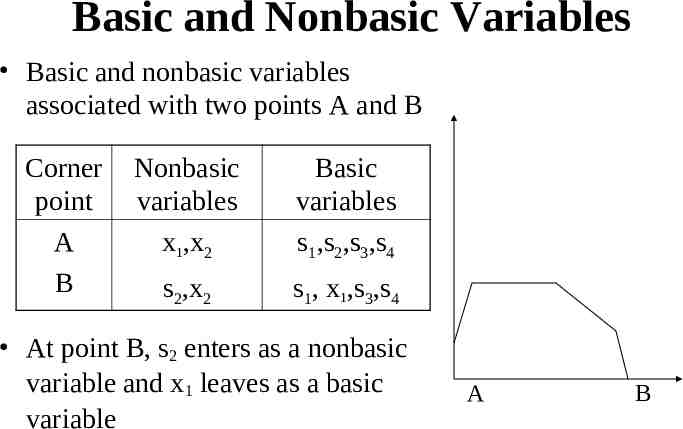
Basic and Nonbasic Variables Basic and nonbasic variables associated with two points A and B Corner point A B Nonbasic variables x1,x2 Basic variables s1,s2,s3,s4 s2,x2 s1, x1,s3,s4 At point B, s2 enters as a nonbasic variable and x1 leaves as a basic variable A B
The Standard Form and the General Concept m equations (m 4) n unknowns (n 6) Sets (n-m) variables to zero and then solves for the remaining m unknowns The variables set equal to zero are called nonbasic variables. The remaining ones are called basic variables At point A, x1 x2 0 which yields s1 6, s2 8, s3 1, and s4 2 At point B, s2 x2 0, which yields x1 4, s1 2, s3 5, and s4 2 Max z 3x1 2x2 0s1 0s2 0s3 0s4 s.t. x1 2x2 s1 6 2x1 x2 -x1 x2 x2 s2 8 s3 1 s4 2 x1,x2,s1,s2,s3,s4 0 A B
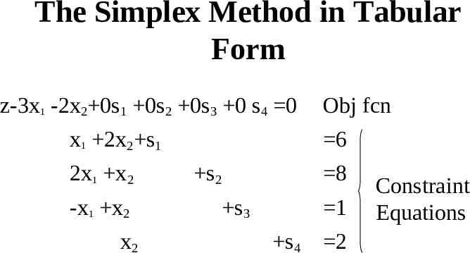
The Simplex Method in Tabular Form z-3x1 -2x2 0s1 0s2 0s3 0 s4 0 x1 2x2 s1 2x1 x2 -x1 x2 x2 Obj fcn 6 s2 8 s3 1 s4 2 Constraint Equations
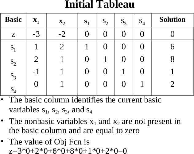
Initial Tableau Basic x1 x2 s1 s2 s3 s4 Solution z s1 -3 1 2 -1 0 -2 2 1 1 1 0 1 0 0 0 0 0 1 0 0 0 0 0 1 0 0 0 0 0 1 0 6 8 1 2 s2 s3 s4 The basic column identifies the current basic variables s1, s2, s3, and s4 The nonbasic variables x1 and x2 are not present in the basic column and are equal to zero The value of Obj Fcn is z 3*0 2*0 6*0 8*0 1*0 2*0 0
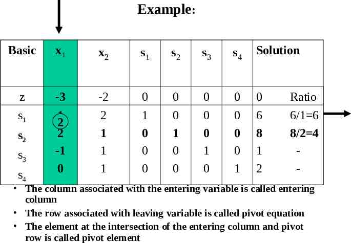
Example: Basic x1 x2 s1 s2 s3 s4 Solution z -3 -2 0 0 0 0 0 Ratio s1 1 2 2 -1 0 2 1 1 1 1 0 0 0 0 1 0 0 0 0 1 0 0 0 0 1 6 8 1 2 6/1 6 8/2 4 - s2 s3 s4 The column associated with the entering variable is called entering column The row associated with leaving variable is called pivot equation The element at the intersection of the entering column and pivot row is called pivot element
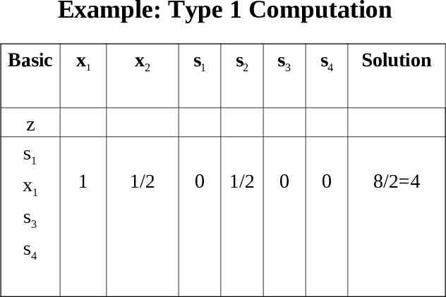
Example: Type 1 Computation Basic x1 x2 s1 s2 s3 s4 Solution 1 1/2 0 1/2 0 0 8/2 4 z s1 x1 s3 s4
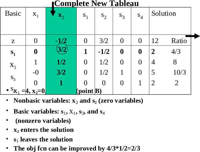
Complete New Tableau Basic x1 x2 s1 s2 s3 s4 Solution z 0 0 3/2 0 0 12 Ratio s1 0 1 -0 0 -1/2 3/2 1 0 0 0 -1/2 1/2 1/2 0 0 0 1 0 0 0 0 1 2 4 5 2 4/3 8 10/3 2 x1 s3 1/2 3/2 1 s4x1 4, x2 0, and z 12 (point B) Nonbasic variables: x2 and s2 (zero variables) Basic variables: s1, x1, s3, and s4 (nonzero variables) x2 enters the solution s1 leaves the solution The obj fcn can be improved by 4/3*1/2 2/3
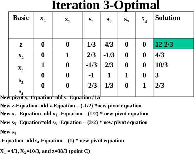
Iteration 3-Optimal Basic x1 x2 s1 s2 s3 s4 Solution z 0 0 1/3 4/3 0 0 12 2/3 x2 0 1 0 0 1 0 0 0 2/3 -1/3 -1/3 2/3 -1 1 -2/3 1/3 0 0 1 0 0 0 0 1 4/3 10/3 3 2/3 x1 s3 s4 New pivot s1-Equation old s1-Equation /1.5 New z-Equation old z-Equation – (-1/2) *new pivot equation New x1 -Equation old x1 -Equation – (1/2) * new pivot equation New s3 -Equation old s3 -Equation – (3/2) * new pivot equation New s4 -Equation old s4-Equation – (1) * new pivot equation x1 4/3, x2 10/3, and z 38/3 (point C)
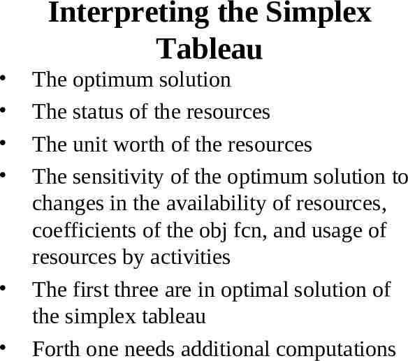
Interpreting the Simplex Tableau The optimum solution The status of the resources The unit worth of the resources The sensitivity of the optimum solution to changes in the availability of resources, coefficients of the obj fcn, and usage of resources by activities The first three are in optimal solution of the simplex tableau Forth one needs additional computations
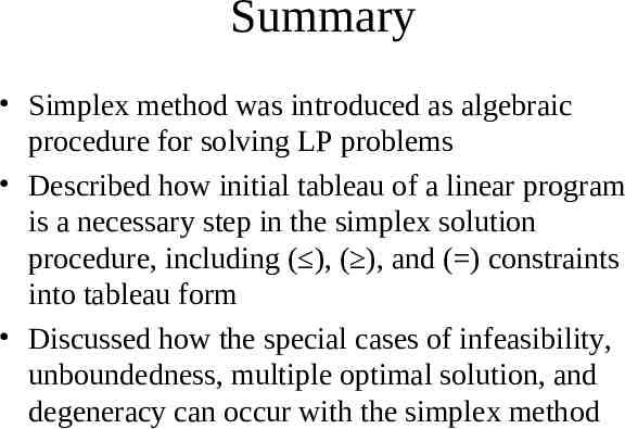
Summary Simplex method was introduced as algebraic procedure for solving LP problems Described how initial tableau of a linear program is a necessary step in the simplex solution procedure, including ( ), ( ), and ( ) constraints into tableau form Discussed how the special cases of infeasibility, unboundedness, multiple optimal solution, and degeneracy can occur with the simplex method
Special Cases in the Simplex Method Special types of LP problems need special attentions Special types: – More than one optimal solution – Infeasible problems – Unbounded solutions – Ties for pivot column and/or ties for the pivot row – Constraints with negative quantity values
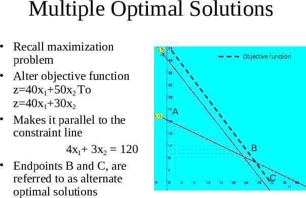
Multiple Optimal Solutions Recall maximization problem Alter objective function z 40x1 50x2 To z 40x1 30x2 Makes it parallel to the constraint line 4x1 3x2 120 Endpoints B and C, are referred to as alternate optimal solutions Objective function A B C
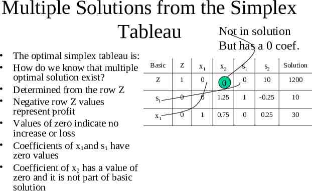
Multiple Solutions from the Simplex Not in solution Tableau The optimal simplex tableau is: How do we know that multiple optimal solution exist? Determined from the row Z Negative row Z values represent profit Values of zero indicate no increase or loss Coefficients of x1and s1 have zero values Coefficient of x2 has a value of zero and it is not part of basic solution But has a 0 coef. Basic Z x1 x2 s1 s2 Solution Z 1 0 0 0 10 1200 s1 0 0 1.25 1 -0.25 10 x1 0 1 0.75 0 0.25 30
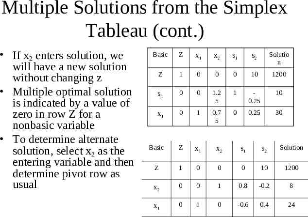
Multiple Solutions from the Simplex Tableau (cont.) If x2 enters solution, we will have a new solution without changing z Multiple optimal solution is indicated by a value of zero in row Z for a nonbasic variable To determine alternate solution, select x2 as the entering variable and then determine pivot row as usual Basic Z x1 x2 s1 s2 Solutio n Z 1 0 0 0 10 1200 s1 0 0 1.2 5 1 0.25 10 x1 0 1 0.7 5 0 0.25 30 Basic Z x1 x2 s1 s2 Solution Z 1 0 0 0 10 1200 x2 0 0 1 0.8 -0.2 8 x1 0 1 0 -0.6 0.4 24
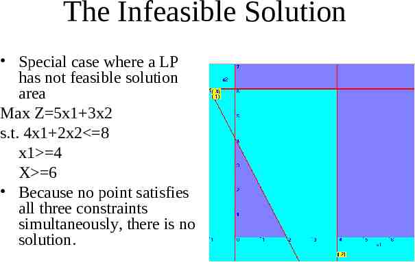
The Infeasible Solution Special case where a LP has not feasible solution area Max Z 5x1 3x2 s.t. 4x1 2x2 8 x1 4 X 6 Because no point satisfies all three constraints simultaneously, there is no solution.
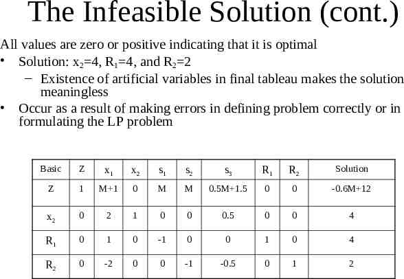
The Infeasible Solution (cont.) All values are zero or positive indicating that it is optimal Solution: x2 4, R1 4, and R2 2 – Existence of artificial variables in final tableau makes the solution meaningless Occur as a result of making errors in defining problem correctly or in formulating the LP problem Basic Z x1 x2 s1 s2 s3 R1 R2 Solution Z 1 M 1 0 M M 0.5M 1.5 0 0 -0.6M 12 x2 0 2 1 0 0 0.5 0 0 4 R1 0 1 0 -1 0 0 1 0 4 R2 0 -2 0 0 -1 -0.5 0 1 2
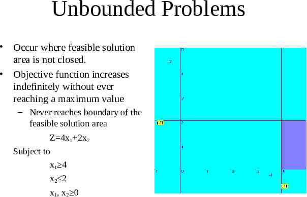
Unbounded Problems Occur where feasible solution area is not closed. Objective function increases indefinitely without ever reaching a maximum value – Never reaches boundary of the feasible solution area Z 4x1 2x2 Subject to x1 4 x2 2 x1, x2 0
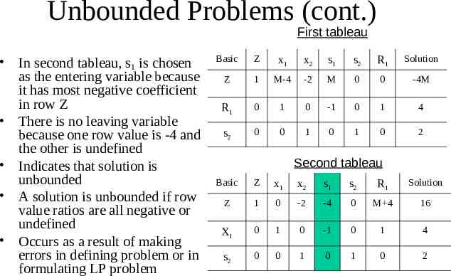
Unbounded Problems (cont.) First tableau In second tableau, s1 is chosen as the entering variable because it has most negative coefficient in row Z There is no leaving variable because one row value is -4 and the other is undefined Indicates that solution is unbounded A solution is unbounded if row value ratios are all negative or undefined Occurs as a result of making errors in defining problem or in formulating LP problem Basic Z x1 x2 s1 s2 R1 Solution Z 1 M-4 -2 M 0 0 -4M R1 0 1 0 -1 0 1 4 s2 0 0 1 0 1 0 2 Second tableau Basic Z x1 x2 s1 s2 R1 Solution Z 1 0 -2 -4 0 M 4 16 X1 0 1 0 -1 0 1 4 s2 0 0 1 0 1 0 2
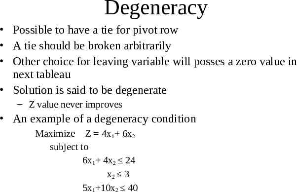
Degeneracy Possible to have a tie for pivot row A tie should be broken arbitrarily Other choice for leaving variable will posses a zero value in next tableau Solution is said to be degenerate – Z value never improves An example of a degeneracy condition Maximize Z 4x1 6x2 subject to 6x1 4x2 24 x2 3 5x1 10x2 40
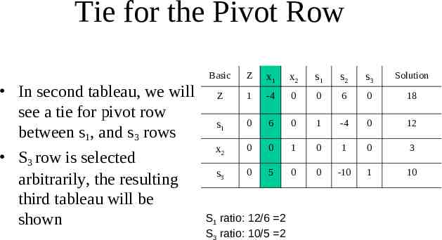
Tie for the Pivot Row In second tableau, we will see a tie for pivot row between s1, and s3 rows S3 row is selected arbitrarily, the resulting third tableau will be shown Basic Z x1 x2 s1 s2 s3 Solution Z 1 -4 0 0 6 0 18 s1 0 6 0 1 -4 0 12 x2 0 0 1 0 1 0 3 s3 0 5 0 0 -10 1 10 S1 ratio: 12/6 2 S3 ratio: 10/5 2
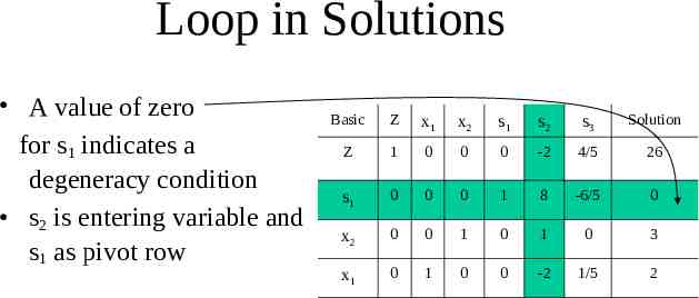
Loop in Solutions A value of zero for s1 indicates a degeneracy condition s2 is entering variable and s1 as pivot row Basic Z x1 x2 s1 s2 s3 Solution Z 1 0 0 0 -2 4/5 26 s1 0 0 0 1 8 -6/5 0 x2 0 0 1 0 1 0 3 x1 0 1 0 0 -2 1/5 2
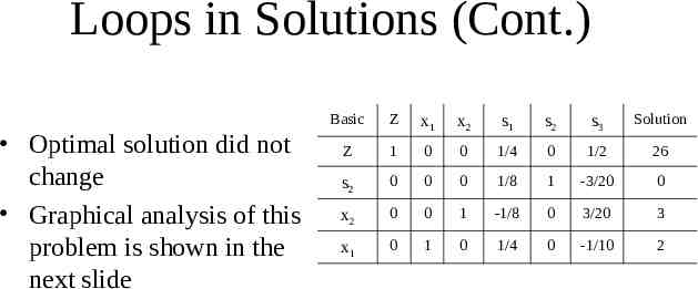
Loops in Solutions (Cont.) Optimal solution did not change Graphical analysis of this problem is shown in the next slide Basic Z x1 x2 s1 s2 s3 Solution Z 1 0 0 1/4 0 1/2 26 s2 0 0 0 1/8 1 -3/20 0 x2 0 0 1 -1/8 0 3/20 3 x1 0 1 0 1/4 0 -1/10 2
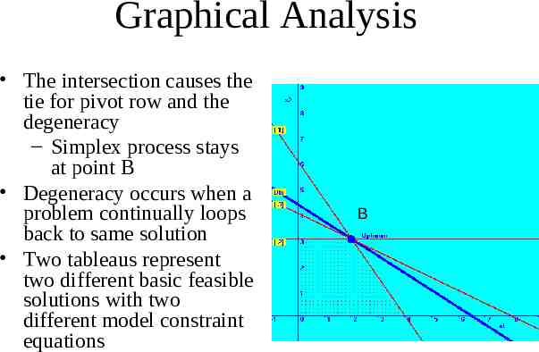
Graphical Analysis The intersection causes the tie for pivot row and the degeneracy – Simplex process stays at point B Degeneracy occurs when a problem continually loops back to same solution Two tableaus represent two different basic feasible solutions with two different model constraint equations B
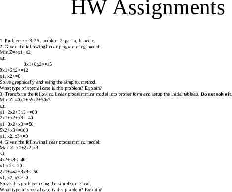
HW Assignments 1. Problem set 3.2A, problem 2, part a, b, and c. 2. Given the following linear programming model: Min Z 4x1 x2 s.t. 3x1 6x2 15 8x1 2x2 12 x1, x2 0 Solve graphically and using the simplex method. What type of special case is this problem? Explain? 3. Transform the following linear programming model into proper form and setup the initial tableau. Do not solve it. Min Z 40x1 55x2 30x3 s.t. x1 2x2 3x3 60 2x1 x2 x3 40 x1 3x2 x3 50 5x2 x3 100 x1, x2, x3 0 4. Given the following linear programming model: Max Z x1 2x2-x3 s.t. 4x2 x3 40 x1-x2 20 2x1 4x2 3x3 60 x1, x2, x3 0 Solve this problem using the simplex method. What type of special case is this problem? Explain?