CS 345: Topics in Data Warehousing Tuesday, October 12, 2004


29 Slides101.50 KB
CS 345: Topics in Data Warehousing Tuesday, October 12, 2004
Review of Thursday’s Class Facts – Semi-additive facts – “Factless” fact tables Slowly Changing Dimensions – Overwrite history – Preserve history – Hybrid schemes More dimension topics – Dimension roles – Junk dimension More fact topics – Multiple currencies – Master/Detail facts and fact allocation – Accumulating Snapshot fact tables
Outline of Today’s Class Customer Relationship Management (CRM) Dimension-focused queries – Drill-across – Conformed dimensions Customer dimension – Behavioral attributes – Auxiliary tables Techniques for very large dimensions – Outriggers – Mini-dimensions Hierarchies – Bridge tables
Customer Relationship Management (CRM) Currently a hot topic in business data analysis Idea: Gain better understanding of customer behavior by integrating data from various sources – Multiple interaction types Orders Returns Customer support Billing Service / repairs – Multiple interaction channels Retail store E-mail Call center (Inbound / Outbound) Web site
CRM questions Customer profitability – Identify most / least profitable customers – 80/20 rule Customer retention – Which customers are most likely to defect to a competitor? – Which retention measures work best? Customer acquisition – Which prospects are most promising? – What offers will entice them to become customers? Up-sell / Cross-sell – Gain additional business from existing customers – Provide targeted offers during “inbound” communications
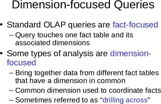
Dimension-focused Queries Standard OLAP queries are fact-focused – Query touches one fact table and its associated dimensions Some types of analysis are dimensionfocused – Bring together data from different fact tables that have a dimension in common – Common dimension used to coordinate facts – Sometimes referred to as “drilling across”
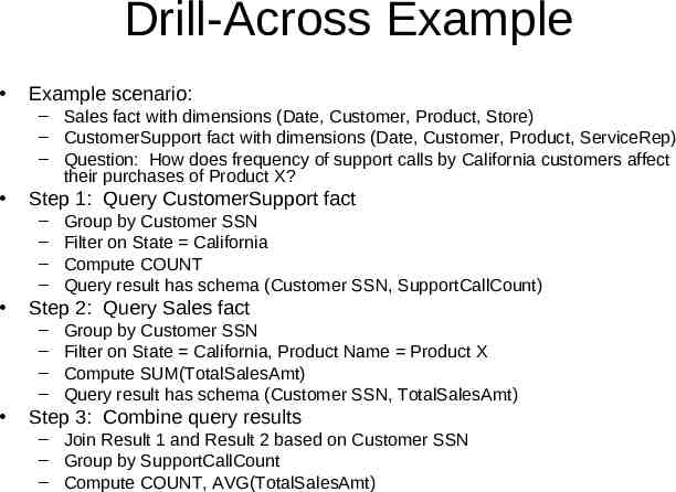
Drill-Across Example Example scenario: – Sales fact with dimensions (Date, Customer, Product, Store) – CustomerSupport fact with dimensions (Date, Customer, Product, ServiceRep) – Question: How does frequency of support calls by California customers affect their purchases of Product X? Step 1: Query CustomerSupport fact – – – – Step 2: Query Sales fact – – – – Group by Customer SSN Filter on State California Compute COUNT Query result has schema (Customer SSN, SupportCallCount) Group by Customer SSN Filter on State California, Product Name Product X Compute SUM(TotalSalesAmt) Query result has schema (Customer SSN, TotalSalesAmt) Step 3: Combine query results – Join Result 1 and Result 2 based on Customer SSN – Group by SupportCallCount – Compute COUNT, AVG(TotalSalesAmt)
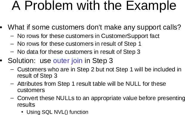
A Problem with the Example What if some customers don’t make any support calls? – No rows for these customers in CustomerSupport fact – No rows for these customers in result of Step 1 – No data for these customers in result of Step 3 Solution: use outer join in Step 3 – Customers who are in Step 2 but not Step 1 will be included in result of Step 3 – Attributes from Step 1 result table will be NULL for these customers – Convert these NULLs to an appropriate value before presenting results Using SQL NVL() function
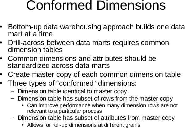
Conformed Dimensions Bottom-up data warehousing approach builds one data mart at a time Drill-across between data marts requires common dimension tables Common dimensions and attributes should be standardized across data marts Create master copy of each common dimension table Three types of “conformed” dimensions: – Dimension table identical to master copy – Dimension table has subset of rows from the master copy Can improve performance when many dimension rows are not relevant to a particular process – Dimension table has subset of attributes from master copy Allows for roll-up dimensions at different grains
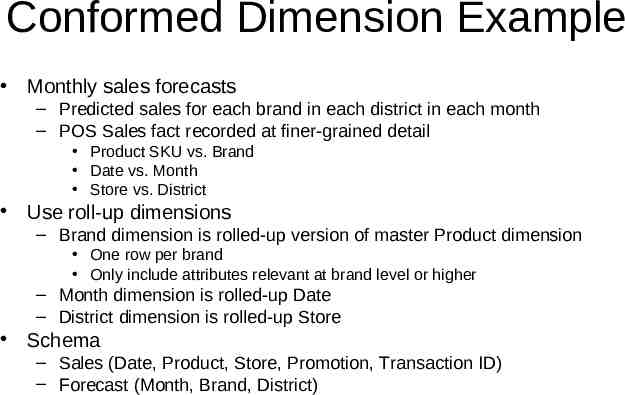
Conformed Dimension Example Monthly sales forecasts – Predicted sales for each brand in each district in each month – POS Sales fact recorded at finer-grained detail Product SKU vs. Brand Date vs. Month Store vs. District Use roll-up dimensions – Brand dimension is rolled-up version of master Product dimension One row per brand Only include attributes relevant at brand level or higher – Month dimension is rolled-up Date – District dimension is rolled-up Store Schema – Sales (Date, Product, Store, Promotion, Transaction ID) – Forecast (Month, Brand, District)
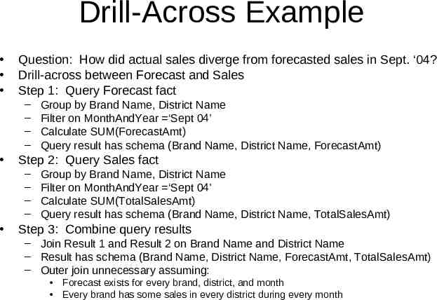
Drill-Across Example Question: How did actual sales diverge from forecasted sales in Sept. ‘04? Drill-across between Forecast and Sales Step 1: Query Forecast fact – – – – Step 2: Query Sales fact – – – – Group by Brand Name, District Name Filter on MonthAndYear ‘Sept 04’ Calculate SUM(ForecastAmt) Query result has schema (Brand Name, District Name, ForecastAmt) Group by Brand Name, District Name Filter on MonthAndYear ‘Sept 04’ Calculate SUM(TotalSalesAmt) Query result has schema (Brand Name, District Name, TotalSalesAmt) Step 3: Combine query results – Join Result 1 and Result 2 on Brand Name and District Name – Result has schema (Brand Name, District Name, ForecastAmt, TotalSalesAmt) – Outer join unnecessary assuming: Forecast exists for every brand, district, and month Every brand has some sales in every district during every month
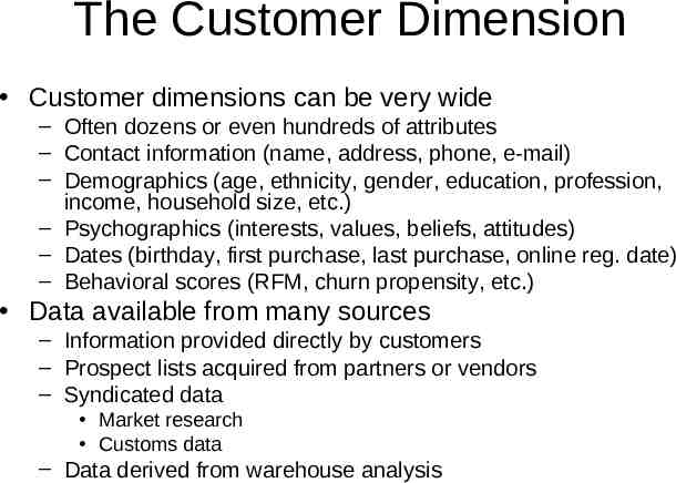
The Customer Dimension Customer dimensions can be very wide – Often dozens or even hundreds of attributes – Contact information (name, address, phone, e-mail) – Demographics (age, ethnicity, gender, education, profession, income, household size, etc.) – Psychographics (interests, values, beliefs, attitudes) – Dates (birthday, first purchase, last purchase, online reg. date) – Behavioral scores (RFM, churn propensity, etc.) Data available from many sources – Information provided directly by customers – Prospect lists acquired from partners or vendors – Syndicated data Market research Customs data – Data derived from warehouse analysis
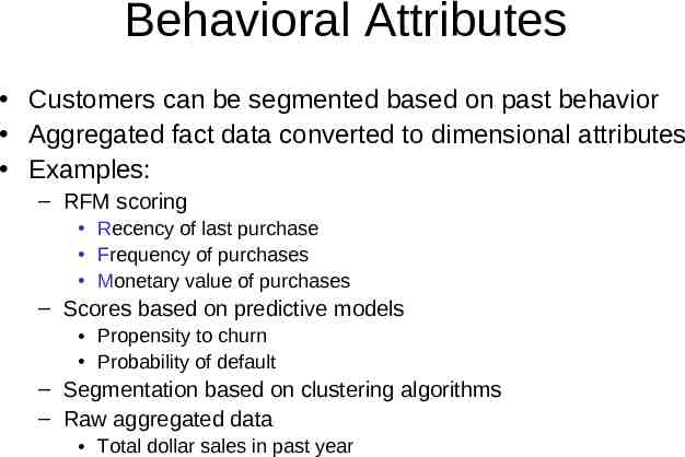
Behavioral Attributes Customers can be segmented based on past behavior Aggregated fact data converted to dimensional attributes Examples: – RFM scoring Recency of last purchase Frequency of purchases Monetary value of purchases – Scores based on predictive models Propensity to churn Probability of default – Segmentation based on clustering algorithms – Raw aggregated data Total dollar sales in past year
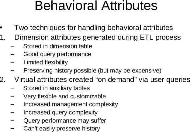
Behavioral Attributes 1. Two techniques for handling behavioral attributes Dimension attributes generated during ETL process – – – – 2. Stored in dimension table Good query performance Limited flexibility Preserving history possible (but may be expensive) Virtual attributes created “on demand” via user queries – – – – – – Stored in auxiliary tables Very flexible and customizable Increased management complexity Increased query complexity Query performance may suffer Can’t easily preserve history
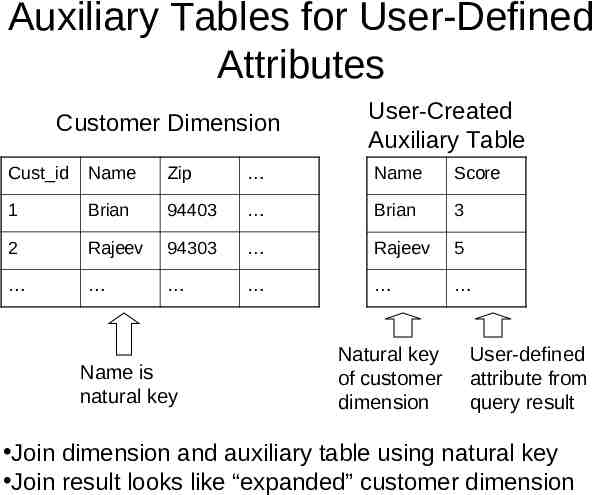
Auxiliary Tables for User-Defined Attributes Customer Dimension User-Created Auxiliary Table Cust id Name Zip Name Score 1 Brian 94403 Brian 3 2 Rajeev 94303 Rajeev 5 Name is natural key Natural key of customer dimension User-defined attribute from query result Join dimension and auxiliary table using natural key Join result looks like “expanded” customer dimension
Another Use of Auxiliary Tables Track a set of customers over time – For example, a focus group or pre-selected sample Set of customers may be defined based on a query Query results may change over time as customer attributes slowly change How to preserve the initial set? Create single-column auxiliary table containing natural key of customers in the set Join to the auxiliary table to filter based on the initial customer set
Continuous vs. Discrete Values Some attributes have large number of possible values on a continuous scale – Income – Age Most simple behavioral attributes are of this type – TotalSalesOfProductXIn2003 Disadvantages of continuous attributes: – Grouping by continuous attribute produces huge, meaningless report – Number of unique attribute combinations explodes Greater number of rows in dimension More frequent changes to value of dimension attributes Group continuous attributes into discrete bands – – – – Like a histogram Instead of Salary 47540, use Salary 40K- 50K Avoids above disadvantages Downside loss of information
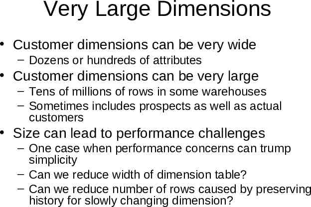
Very Large Dimensions Customer dimensions can be very wide – Dozens or hundreds of attributes Customer dimensions can be very large – Tens of millions of rows in some warehouses – Sometimes includes prospects as well as actual customers Size can lead to performance challenges – One case when performance concerns can trump simplicity – Can we reduce width of dimension table? – Can we reduce number of rows caused by preserving history for slowly changing dimension?
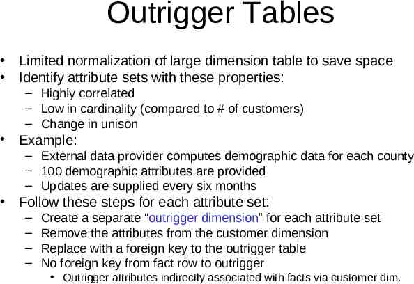
Outrigger Tables Limited normalization of large dimension table to save space Identify attribute sets with these properties: – Highly correlated – Low in cardinality (compared to # of customers) – Change in unison Example: – External data provider computes demographic data for each county – 100 demographic attributes are provided – Updates are supplied every six months Follow these steps for each attribute set: – – – – Create a separate “outrigger dimension” for each attribute set Remove the attributes from the customer dimension Replace with a foreign key to the outrigger table No foreign key from fact row to outrigger Outrigger attributes indirectly associated with facts via customer dim.
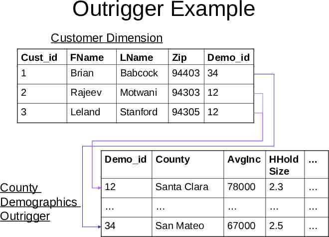
Outrigger Example Customer Dimension Cust id FName LName Zip 1 Brian Babcock 94403 34 2 Rajeev Motwani 94303 12 3 Leland Stanford 94305 12 County Demographics Outrigger Demo id Demo id County AvgInc HHold Size 12 Santa Clara 78000 2.3 34 San Mateo 67000 2.5
Outrigger Tables Advantages: – Space savings Customer dimension table becomes narrower Outrigger table has relatively few rows One copy per county vs. one copy per customer Disadvantages: – Additional tables introduced Accessing outrigger attributes requires an extra join Users must remember which attributes are in outrigger vs. main customer dimension – Creating a view can solve this problem
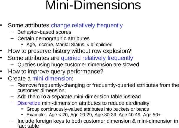
Mini-Dimensions Some attributes change relatively frequently – Behavior-based scores – Certain demographic attributes Age, Income, Marital Status, # of children How to preserve history without row explosion? Some attributes are queried relatively frequently – Queries using huge customer dimension are slowed How to improve query performance? Create a mini-dimension: – Remove frequently-changing or frequently-queried attributes from the customer dimension – Add them to a separate mini-dimension table instead – Discretize mini-dimension attributes to reduce cardinality Group continuously-valued attributes into buckets or bands Example: Age 20, Age 20-29, Age 30-39, Age 40-49, Age 50 – Include foreign keys to both customer dimension & mini-dimension in fact table
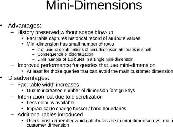
Mini-Dimensions Advantages: – History preserved without space blow-up Fact table captures historical record of attribute values Mini-dimension has small number of rows – # of unique combinations of mini-dimension attributes is small – Consequence of discretization – Limit number of attributes in a single mini-dimension! – Improved performance for queries that use mini-dimension At least for those queries that can avoid the main customer dimension Disadvantages: – Fact table width increases Due to increased number of dimension foreign keys – Information lost due to discretization Less detail is available Impractical to change bucket / band boundaries – Additional tables introduced Users must remember which attributes are in mini-dimension vs. main customer dimension
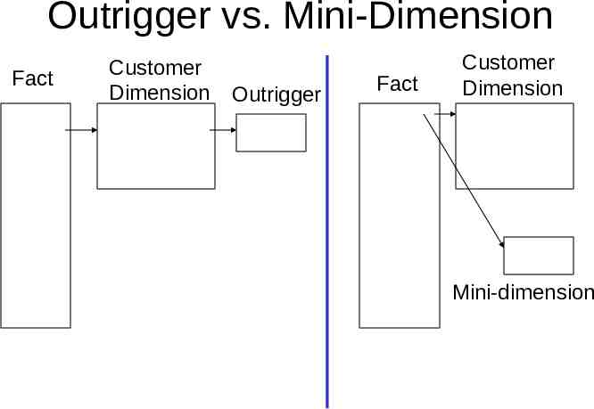
Outrigger vs. Mini-Dimension Fact Customer Dimension Outrigger Fact Customer Dimension Mini-dimension
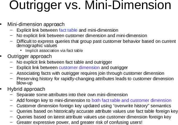
Outrigger vs. Mini-Dimension Mini-dimension approach – Explicit link between fact table and mini-dimension – No explicit link between customer dimension and mini-dimension – Difficult to express queries that group past customer behavior based on current demographic values Implicit association via fact table Outrigger approach – – – – No explicit link between fact table and outrigger Explicit link between customer dimension and outrigger Associating facts with outrigger requires join through customer dimension Preserving history for rapidly-changing attributes leads to customer dimension blow-up Hybrid approach – – – – – – Separate some attributes into their own mini-dimension Add foreign key to mini-dimension to both fact table and customer dimension Customer dimension foreign key updated using “overwrite history” semantics Queries based on historically accurate attribute values use fact table foreign key Queries based on latest attribute values use customer dimension foreign key Greater expressive power, and greater risk of confusing users!
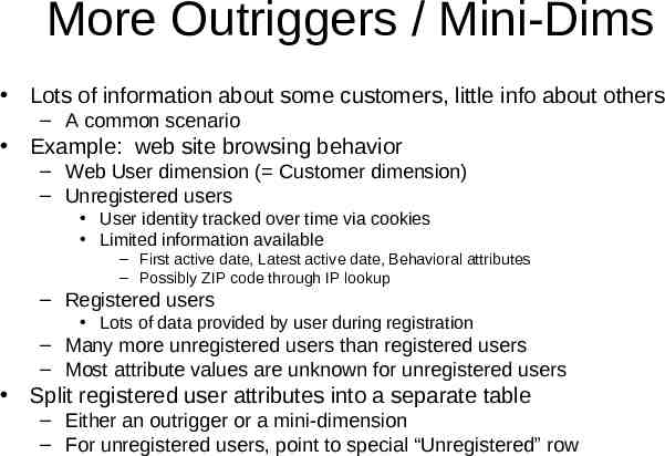
More Outriggers / Mini-Dims Lots of information about some customers, little info about others – A common scenario Example: web site browsing behavior – Web User dimension ( Customer dimension) – Unregistered users User identity tracked over time via cookies Limited information available – First active date, Latest active date, Behavioral attributes – Possibly ZIP code through IP lookup – Registered users Lots of data provided by user during registration – Many more unregistered users than registered users – Most attribute values are unknown for unregistered users Split registered user attributes into a separate table – Either an outrigger or a mini-dimension – For unregistered users, point to special “Unregistered” row
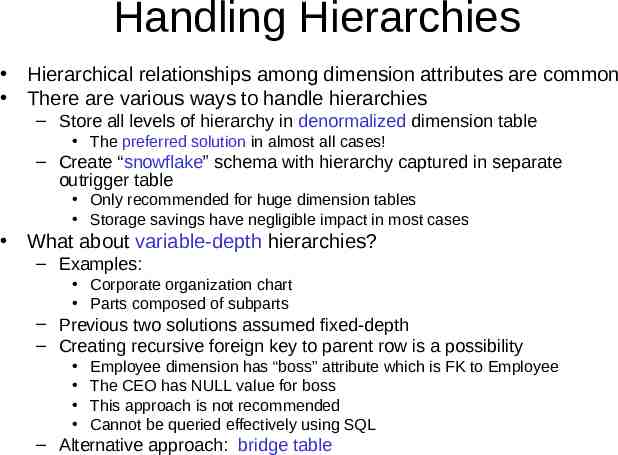
Handling Hierarchies Hierarchical relationships among dimension attributes are common There are various ways to handle hierarchies – Store all levels of hierarchy in denormalized dimension table The preferred solution in almost all cases! – Create “snowflake” schema with hierarchy captured in separate outrigger table Only recommended for huge dimension tables Storage savings have negligible impact in most cases What about variable-depth hierarchies? – Examples: Corporate organization chart Parts composed of subparts – Previous two solutions assumed fixed-depth – Creating recursive foreign key to parent row is a possibility Employee dimension has “boss” attribute which is FK to Employee The CEO has NULL value for boss This approach is not recommended Cannot be queried effectively using SQL – Alternative approach: bridge table
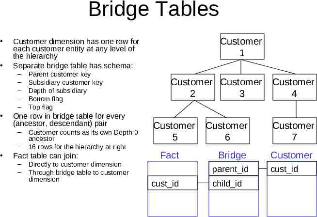
Bridge Tables – – – – – Parent customer key Subsidiary customer key Depth of subsidiary Bottom flag Top flag One row in bridge table for every (ancestor, descendant) pair – – Customer 1 Customer dimension has one row for each customer entity at any level of the hierarchy Separate bridge table has schema: Customer counts as its own Depth-0 ancestor 16 rows for the hierarchy at right Fact table can join: – – Directly to customer dimension Through bridge table to customer dimension Customer Customer 2 3 Customer 5 Fact Customer 6 Customer 7 Bridge Customer parent id cust id Customer 4 child id cust id
Using Bridge Tables in Queries Two join directions – Navigate up the hierarchy Fact joins to subsidiary customer key Dimension joins to parent customer key – Navigate down the hierarchy Fact joins to parent customer key Dimension joins to subsidiary customer key Safe uses of the bridge table: – Filter on customer dimension restricts query to a single customer Use bridge table to combine data about that customer’s subsidiaries or parents – Filter on bridge table restricts query to a single level Require Top Flag Y Require Depth 1 – For immediate parent / child organizations Require (Depth 1 OR Top Flag Y) – Generalizes the previous example to properly treat top-level customers Other uses of the bridge table risk over-counting – Bridge table is many-to-many between fact and dimension