Correlation and Regression Cal State Northridge 427 Ainsworth

81 Slides1.67 MB
Correlation and Regression Cal State Northridge 427 Ainsworth
Major Points - Correlation Questions answered by correlation Scatterplots An example The correlation coefficient Other kinds of correlations Factors affecting correlations Testing for significance
The Question Are two variables related? Does one increase as the other increases? e. Does one decrease as the other increases? e. g. skills and income g. health problems and nutrition How can we get a numerical measure of the degree of relationship?
Scatterplots AKA scatter diagram or scattergram. Graphically depicts the relationship between two variables in two dimensional space.
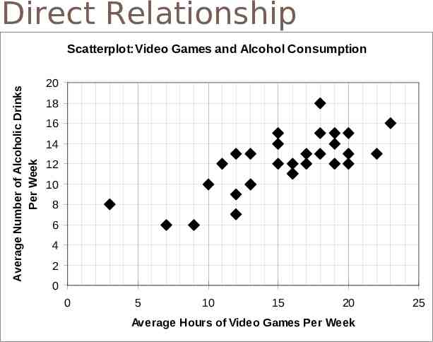
Direct Relationship Average Number of Alcoholic Drinks Per Week Scatterplot:Video Games and Alcohol Consumption 20 18 16 14 12 10 8 6 4 2 0 0 5 10 15 20 Average Hours of Video Games Per Week 25
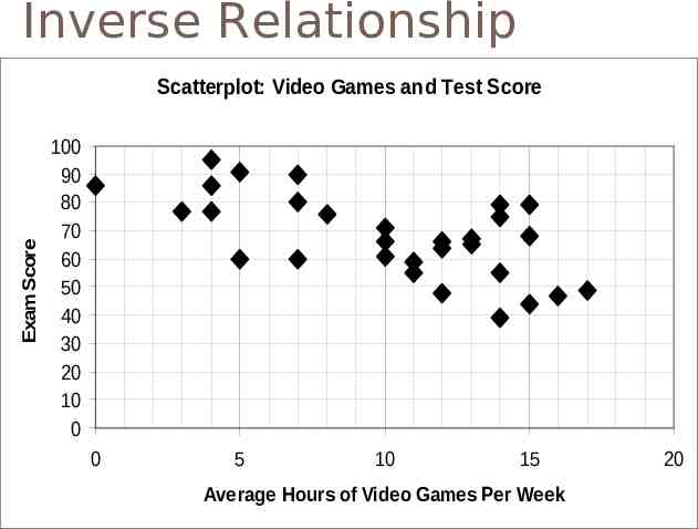
Inverse Relationship Exam Score Scatterplot: Video Games and Test Score 100 90 80 70 60 50 40 30 20 10 0 0 5 10 15 Average Hours of Video Games Per Week 20
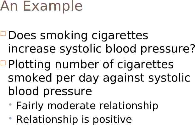
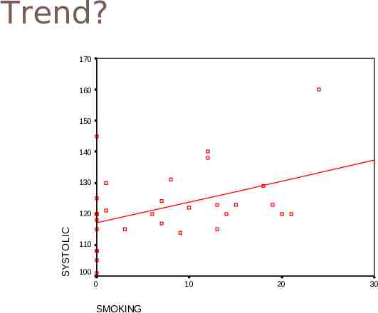
An Example Does smoking cigarettes increase systolic blood pressure? Plotting number of cigarettes smoked per day against systolic blood pressure Fairly moderate relationship Relationship is positive
Trend? 170 160 150 140 130 SYSTOLIC 120 110 100 0 SMOKING 10 20 30
Smoking and BP Note relationship is moderate, but real. Why do we care about relationship? What would conclude if there were no relationship? What if the relationship were near perfect? What if the relationship were negative?
Heart Disease and Cigarettes Data on heart disease and cigarette smoking in 21 developed countries (Landwehr and Watkins, 1987) Data have been rounded for computational convenience. The results were not affected.
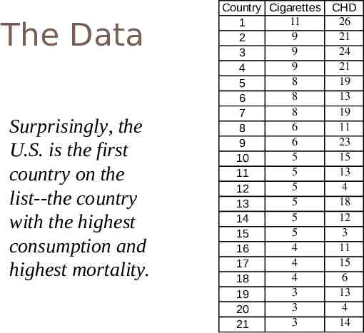
The Data Surprisingly, the U.S. is the first country on the list--the country with the highest consumption and highest mortality. Country Cigarettes CHD 11 26 1 9 21 2 9 24 3 9 21 4 8 19 5 8 13 6 8 19 7 6 11 8 6 23 9 5 15 10 5 13 11 5 4 12 5 18 13 5 12 14 5 3 15 4 11 16 4 15 17 4 6 18 3 13 19 3 4 20 3 14 21
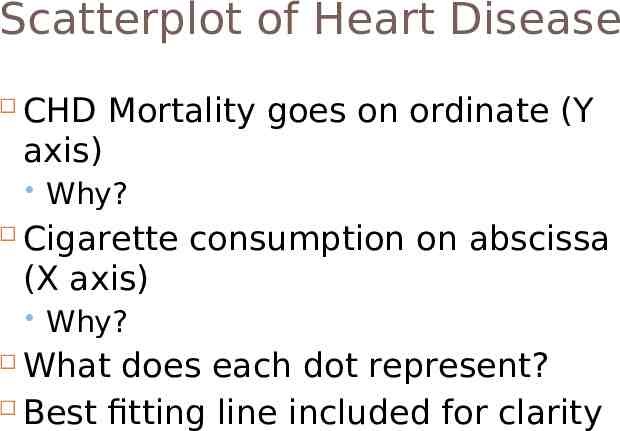
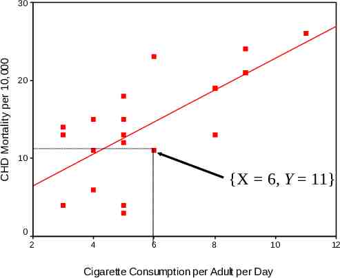
Scatterplot of Heart Disease CHD Mortality goes on ordinate (Y axis) Why? Cigarette consumption on abscissa (X axis) Why? What does each dot represent? Best fitting line included for clarity
CHD Mortality per 10,000 30 20 10 {X 6, Y 11} 0 2 4 6 8 10 Cigarette Consumption per Adult per Day 12
What Does the Scatterplot Show? As smoking increases, so does coronary heart disease mortality. Relationship looks strong Not all data points on line. This gives us “residuals” or “errors of prediction” To be discussed later
Correlation Co-relation The relationship between two variables Measured with a correlation coefficient Most popularly seen correlation coefficient: Pearson ProductMoment Correlation
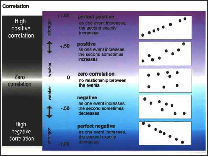
Types of Correlation Positive correlation High values of X tend to be associated with high values of Y. As X increases, Y increases Negative correlation High values of X tend to be associated with low values of Y. As X increases, Y decreases No correlation No consistent tendency for values on Y to increase or decrease as X increases
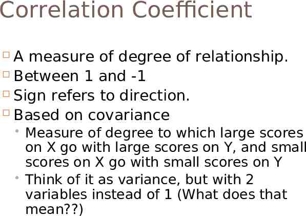
Correlation Coefficient A measure of degree of relationship. Between 1 and -1 Sign refers to direction. Based on covariance Measure of degree to which large scores on X go with large scores on Y, and small scores on X go with small scores on Y Think of it as variance, but with 2 variables instead of 1 (What does that mean?)
18
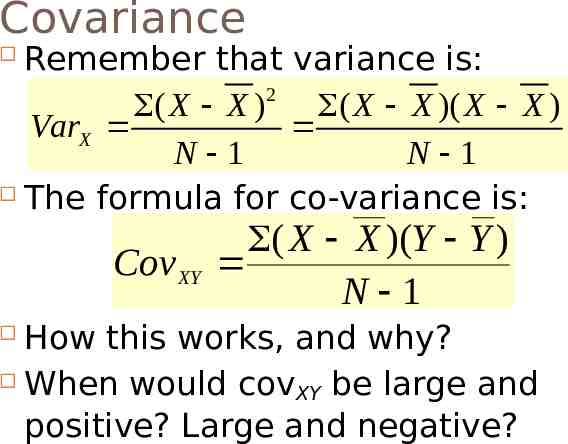
Covariance Remember that variance is: 2 ( X X ) ( X X )( X X ) VarX N 1 N 1 The formula for co-variance is: Cov XY ( X X )(Y Y ) N 1 How this works, and why? When would cov XY be large and positive? Large and negative?
Example
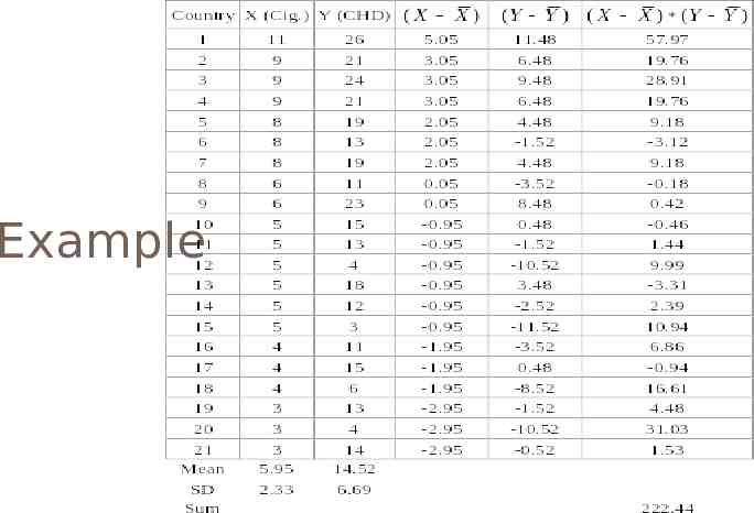
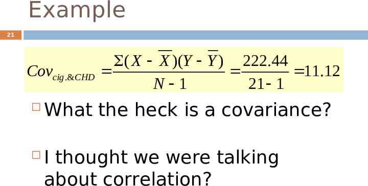
Example 21 Covcig .&CHD ( X X )(Y Y ) 222.44 11.12 N 1 21 1 What the heck is a covariance? I thought we were talking about correlation?
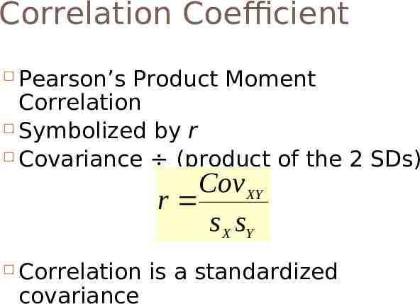
Correlation Coefficient Pearson’s Product Moment Correlation Symbolized by r Covariance (product of the 2 SDs) Cov XY r s X sY Correlation is a standardized covariance
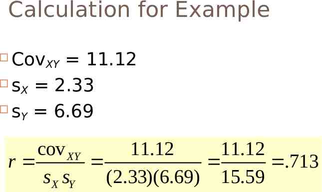
Calculation for Example CovXY 11.12 s 2.33 X s 6.69 Y cov XY 11.12 11.12 r .713 s X sY (2.33)(6.69) 15.59
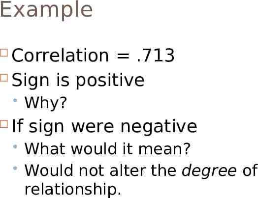
Example Correlation .713 Sign is positive Why? If sign were negative What would it mean? Would not alter the degree of relationship.
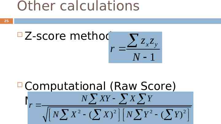
Other calculations 25 Z-score method zx z y r N 1 Computational (Raw Score) N XY X Y Method r N X 2 ( X ) 2 N Y 2 ( Y ) 2
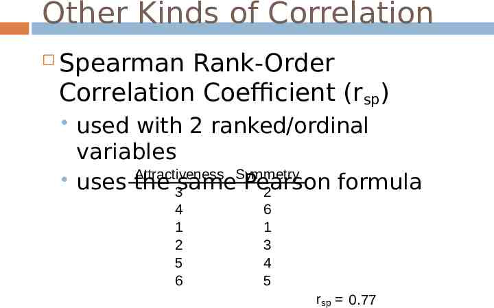
Other Kinds of Correlation Spearman Rank-Order Correlation Coefficient (rsp) used with 2 ranked/ordinal variables Attractiveness Symmetry uses the 3same Pearson formula 2 4 1 2 5 6 6 1 3 4 5 rsp 0.77 26
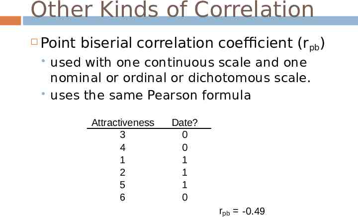
Other Kinds of Correlation Point biserial correlation coefficient (rpb) used with one continuous scale and one nominal or ordinal or dichotomous scale. uses the same Pearson formula Attractiveness 3 4 1 2 5 6 Date? 0 0 1 1 1 0 rpb -0.49 27
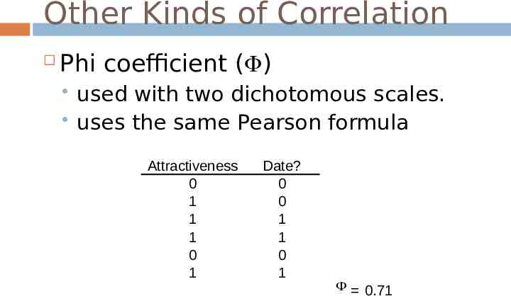
Other Kinds of Correlation Phi coefficient ( ) used with two dichotomous scales. uses the same Pearson formula Attractiveness 0 1 1 1 0 1 Date? 0 0 1 1 0 1 F 0.71 28
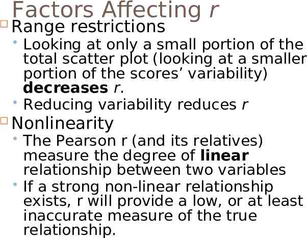
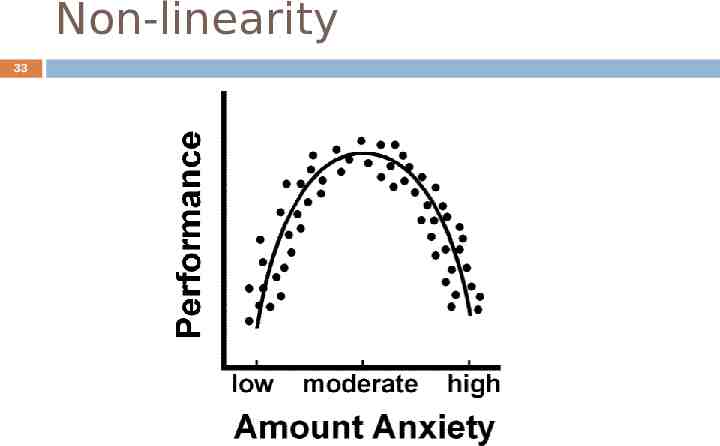
Factors Affecting r Range restrictions Looking at only a small portion of the total scatter plot (looking at a smaller portion of the scores’ variability) decreases r. Reducing variability reduces r Nonlinearity The Pearson r (and its relatives) measure the degree of linear relationship between two variables If a strong non-linear relationship exists, r will provide a low, or at least inaccurate measure of the true relationship.
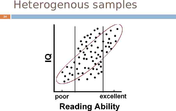
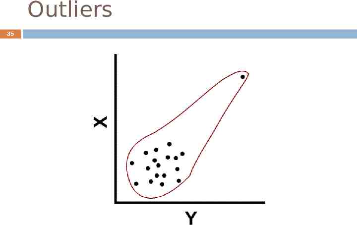
Factors Affecting r Heterogeneous subsamples Everyday examples (e.g. height and weight using both men and women) Outliers Overestimate Correlation Underestimate Correlation
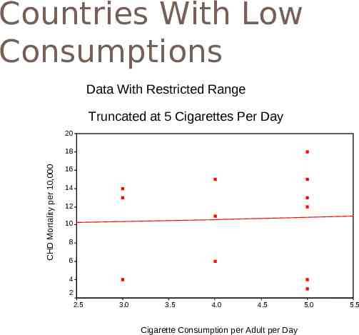
Countries With Low Consumptions Data With Restricted Range Truncated at 5 Cigarettes Per Day 20 CHD Mortality per 10,000 18 16 14 12 10 8 6 4 2 2.5 3.0 3.5 4.0 4.5 Cigarette Consumption per Adult per Day 5.0 5.5
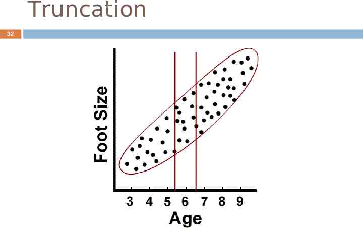
Truncation 32
Non-linearity 33
Heterogenous samples 34
Outliers 35
Testing Correlations 36 So you have a correlation. Now what? In terms of magnitude, how big is big? Small correlations in large samples are “big.” Large correlations in small samples aren’t always “big.” Depends upon the magnitude of the correlation coefficient AND The size of your sample.
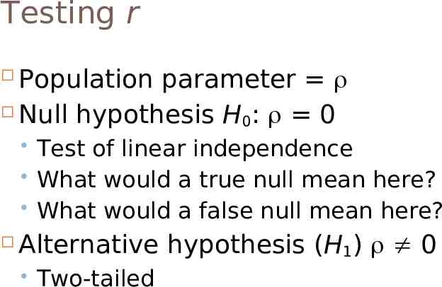
Testing r Population parameter Null hypothesis H : 0 0 Test of linear independence What would a true null mean here? What would a false null mean here? Alternative hypothesis (H1) 0 Two-tailed
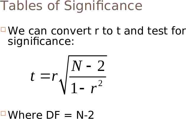
Tables of Significance We can convert r to t and test for significance: N 2 t r 2 1 r Where DF N-2
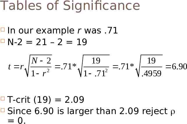
Tables of Significance In our example r was .71 N-2 21 – 2 19 N 2 19 19 t r .71* .71* 6.90 2 2 1 r 1 .71 .4959 T-crit (19) 2.09 Since 6.90 is larger than 2.09 reject 0.
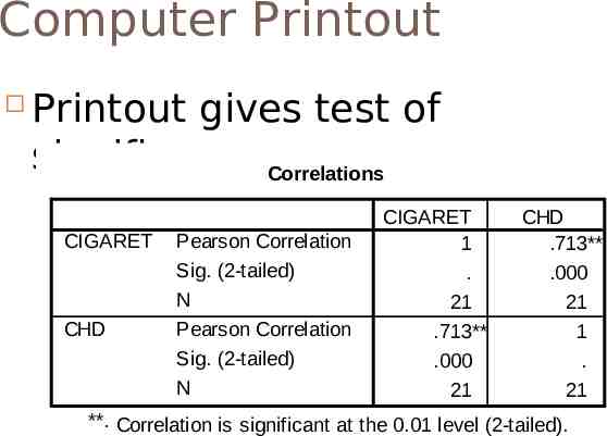
Computer Printout Printout gives test of significance.Correlations CIGARET CHD Pearson Correlation Sig. (2-tailed) N Pearson Correlation Sig. (2-tailed) N CIGARET 1 . 21 .713** .000 21 CHD .713** .000 21 1 . 21 **. Correlation is significant at the 0.01 level (2-tailed).
Regression
What is regression? 42 How do we predict one variable from another? How does one variable change as the other changes? Influence
Linear Regression 43 A technique we use to predict the most likely score on one variable from those on another variable Uses the nature of the relationship (i.e. correlation) between two variables to enhance your prediction
Linear Regression: Parts 44 Y - the variables you are predicting X - the variables you are using to predict i.e. dependent variable i.e. independent variable Ŷ - your predictions (also known as Y’)
Why Do We Care? 45 We may want to make a prediction. More likely, we want to understand the relationship. How fast does CHD mortality rise with a one unit increase in smoking? Note: we speak about predicting, but often don’t actually predict.
An Example 46 Cigarettes and CHD Mortality again Data repeated on next slide We want to predict level of CHD mortality in a country averaging 10 cigarettes per day.
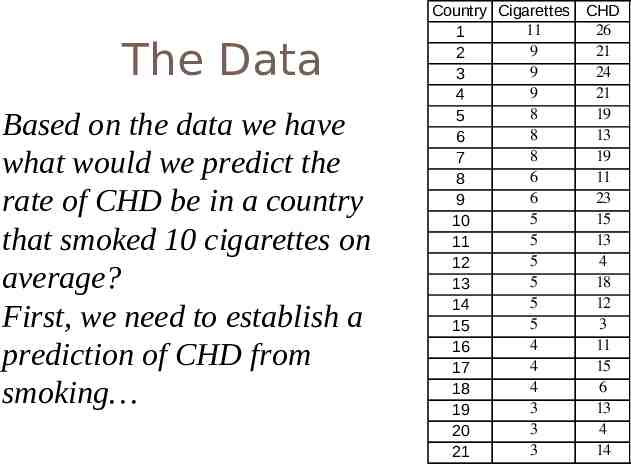
47 The Data Based on the data we have what would we predict the rate of CHD be in a country that smoked 10 cigarettes on average? First, we need to establish a prediction of CHD from smoking Country Cigarettes CHD 11 26 1 9 21 2 9 24 3 9 21 4 8 19 5 8 13 6 8 19 7 6 11 8 6 23 9 5 15 10 5 13 11 5 4 12 5 18 13 5 12 14 5 3 15 4 11 16 4 15 17 4 6 18 3 13 19 3 4 20 3 14 21
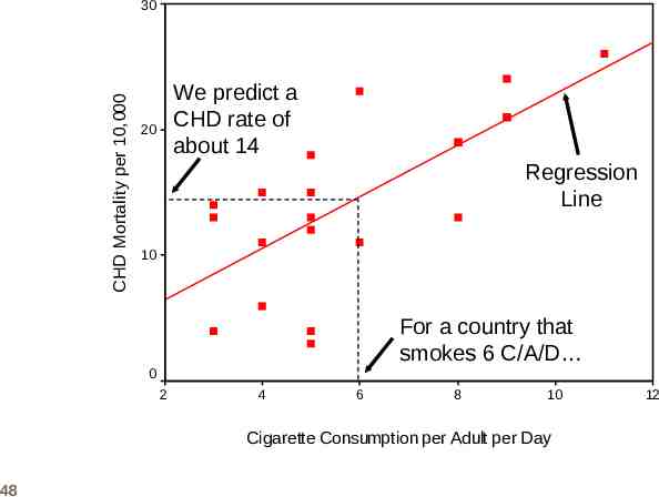
CHD Mortality per 10,000 30 We predict a CHD rate of about 14 20 Regression Line 10 For a country that smokes 6 C/A/D 0 2 4 6 8 10 Cigarette Consumption per Adult per Day 48 12
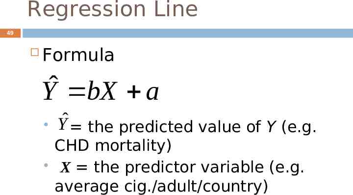
Regression Line 49 Formula Yˆ bX a Yˆ the predicted value of Y (e.g. CHD mortality) X the predictor variable (e.g. average cig./adult/country)
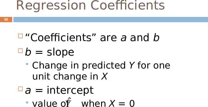
Regression Coefficients 50 “Coefficients” are a and b b slope Change in predicted Y for one unit change in X a intercept value ofYˆ when X 0
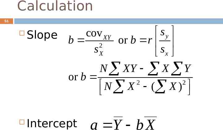
Calculation 51 Slope b cov XY or b r s y 2 sX sx or b Intercept N XY N X 2 X Y ( X ) a Y b X 2
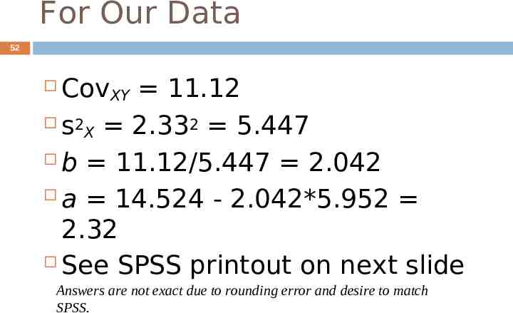
For Our Data 52 CovXY 11.12 s2 2.332 5.447 X b 11.12/5.447 2.042 a 14.524 - 2.042*5.952 2.32 See SPSS printout on next slide Answers are not exact due to rounding error and desire to match SPSS.
SPSS Printout 53
Note: 54 The values we obtained are shown on printout. The intercept is the value in the B column labeled “constant” The slope is the value in the B column labeled by name of predictor variable.
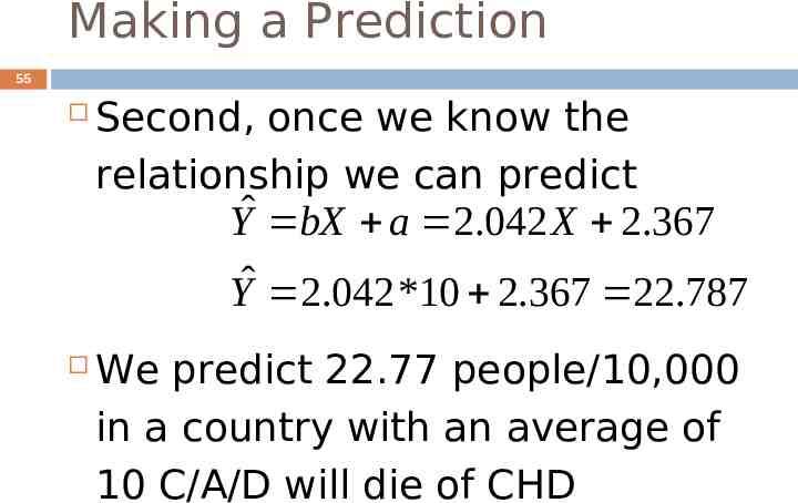
Making a Prediction 55 Second, once we know the relationship we can predict Yˆ bX a 2.042 X 2.367 Yˆ 2.042*10 2.367 22.787 We predict 22.77 people/10,000 in a country with an average of 10 C/A/D will die of CHD
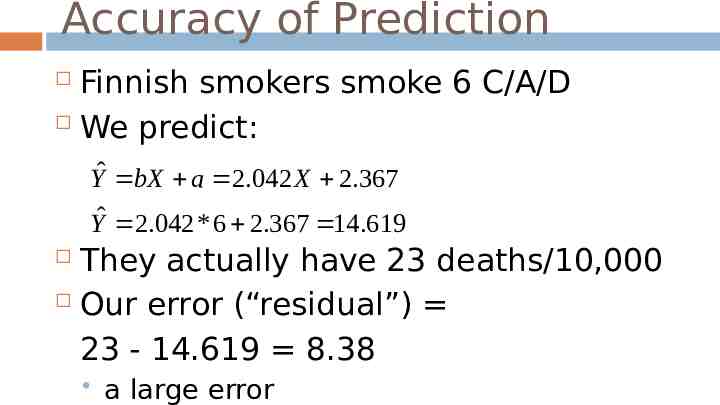
Accuracy of Prediction Finnish smokers smoke 6 C/A/D We predict: Yˆ bX a 2.042 X 2.367 Yˆ 2.042*6 2.367 14.619 They actually have 23 deaths/10,000 Our error (“residual”) 23 - 14.619 8.38 a large error 56
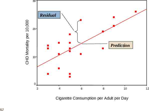
30 CHD Mortality per 10,000 Residual 20 Prediction 10 0 2 4 6 8 10 Cigarette Consumption per Adult per Day 57 12
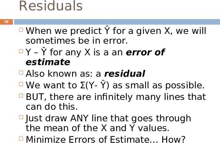
Residuals 58 When we predict Ŷ for a given X, we will sometimes be in error. Y – Ŷ for any X is a an error of estimate Also known as: a residual We want to Σ(Y- Ŷ) as small as possible. BUT, there are infinitely many lines that can do this. Just draw ANY line that goes through the mean of the X and Y values. Minimize Errors of Estimate How?
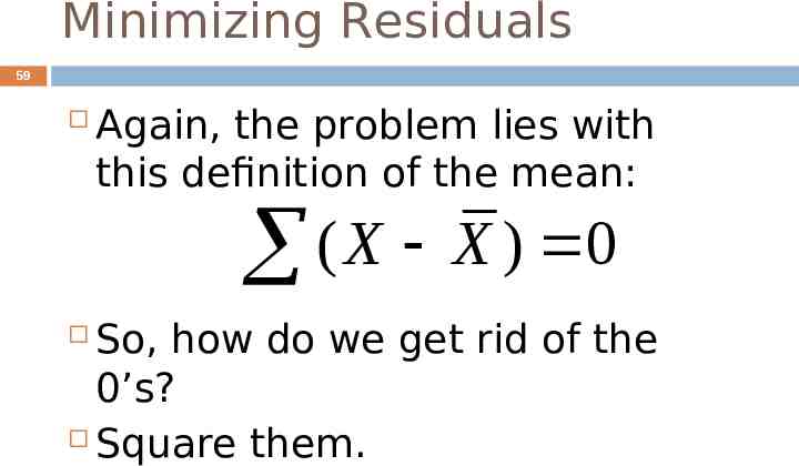
Minimizing Residuals 59 Again, the problem lies with this definition of the mean: (X X ) 0 So, how do we get rid of the 0’s? Square them.
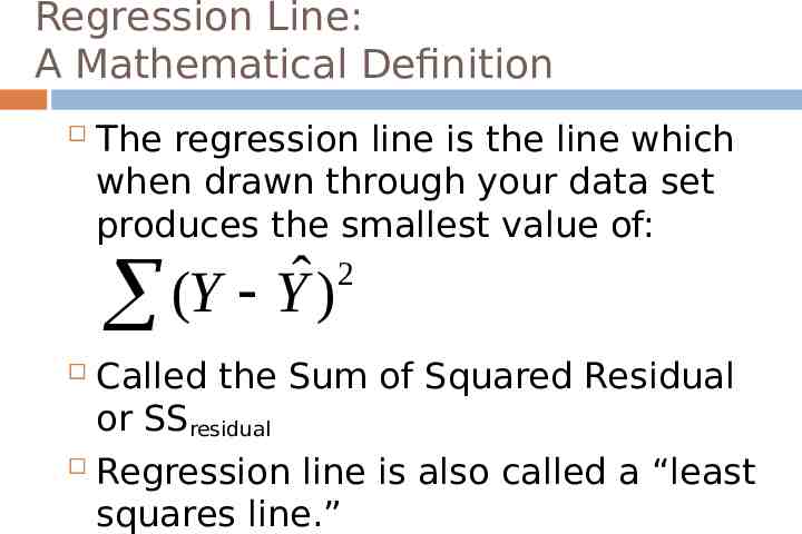
Regression Line: A Mathematical Definition The regression line is the line which when drawn through your data set produces the smallest value of: 2 ˆ (Y Y ) Called the Sum of Squared Residual or SSresidual Regression line is also called a “least 60 squares line.”
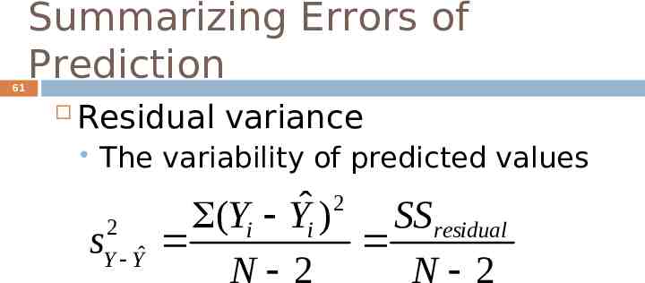
61 Summarizing Errors of Prediction Residual variance The variability of predicted values 2 Y Yˆ s 2 ˆ (Yi Yi ) SS residual N 2 N 2
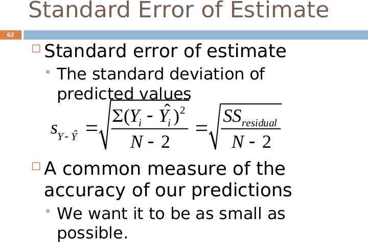
Standard Error of Estimate 62 Standard error of estimate The standard deviation of predicted values 2 ˆ (Yi Yi ) SS residual sY Yˆ N 2 N 2 A common measure of the accuracy of our predictions We want it to be as small as possible.
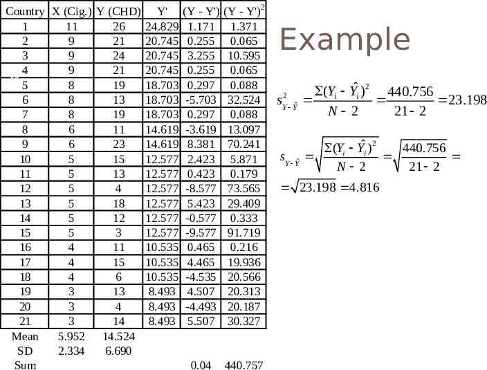
Country X (Cig.) Y (CHD) 1 11 26 2 9 21 3 9 24 9 21 63 4 5 8 19 6 8 13 7 8 19 8 6 11 9 6 23 10 5 15 11 5 13 12 5 4 13 5 18 14 5 12 15 5 3 16 4 11 17 4 15 18 4 6 19 3 13 20 3 4 21 3 14 Mean 5.952 14.524 SD 2.334 6.690 Sum Y' 24.829 20.745 20.745 20.745 18.703 18.703 18.703 14.619 14.619 12.577 12.577 12.577 12.577 12.577 12.577 10.535 10.535 10.535 8.493 8.493 8.493 (Y - Y') 1.171 0.255 3.255 0.255 0.297 -5.703 0.297 -3.619 8.381 2.423 0.423 -8.577 5.423 -0.577 -9.577 0.465 4.465 -4.535 4.507 -4.493 5.507 (Y - Y')2 1.371 0.065 10.595 0.065 0.088 32.524 0.088 13.097 70.241 5.871 0.179 73.565 29.409 0.333 91.719 0.216 19.936 20.566 20.313 20.187 30.327 0.04 440.757 Example 2 Y Yˆ s (Yi Yˆi )2 440.756 23.198 N 2 21 2 sY Yˆ (Yi Yˆi ) 2 440.756 N 2 21 2 23.198 4.816
Regression and Z Scores 64 When your data are standardized (linearly transformed to z-scores), the slope of the regression line is called β DO NOT confuse this β with the β associated with type II errors. They’re different. When we have one predictor, r β Z βZ , since A now equals 0 y x
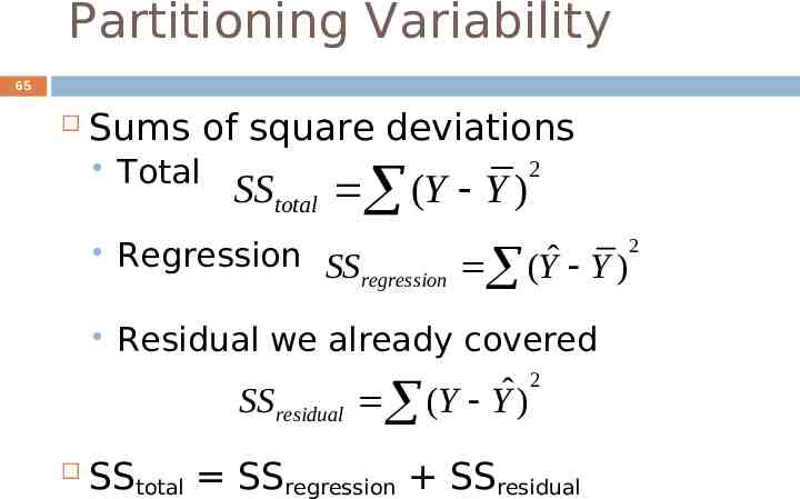
Partitioning Variability 65 Sums of square deviations Total SStotal (Y Y ) Regression SS ˆ ( Y Y) regression Residual we already covered SS residual (Y Yˆ ) 2 2 SStotal SSregression SSresidual 2
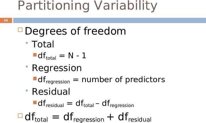
Partitioning Variability 66 Degrees of freedom Total dftotal N-1 Regression dfregression Residual dfresidual number of predictors dftotal – dfregression dftotal dfregression dfresidual
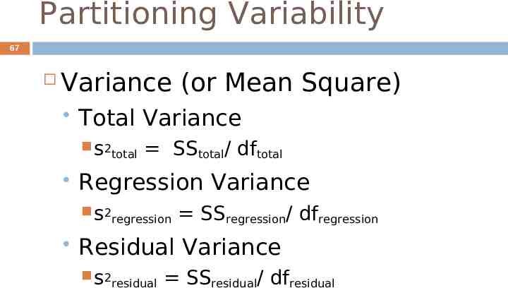
Partitioning Variability 67 Variance (or Mean Square) Total Variance s2total SStotal/ dftotal Regression Variance s2regression SSregression/ dfregression Residual Variance s2residual SSresidual/ dfresidual
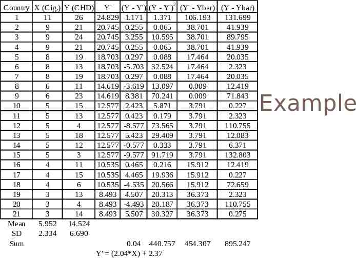
Country X (Cig.) Y (CHD) 1 11 26 2 9 21 3 9 24 68 4 9 21 5 8 19 6 8 13 7 8 19 8 6 11 9 6 23 10 5 15 11 5 13 12 5 4 13 5 18 14 5 12 15 5 3 16 4 11 17 4 15 18 4 6 19 3 13 20 3 4 21 3 14 Mean 5.952 14.524 SD 2.334 6.690 Sum Y' 24.829 20.745 20.745 20.745 18.703 18.703 18.703 14.619 14.619 12.577 12.577 12.577 12.577 12.577 12.577 10.535 10.535 10.535 8.493 8.493 8.493 (Y - Y') 1.171 0.255 3.255 0.255 0.297 -5.703 0.297 -3.619 8.381 2.423 0.423 -8.577 5.423 -0.577 -9.577 0.465 4.465 -4.535 4.507 -4.493 5.507 (Y - Y')2 (Y' - Ybar) (Y - Ybar) 1.371 106.193 131.699 0.065 38.701 41.939 10.595 38.701 89.795 0.065 38.701 41.939 0.088 17.464 20.035 32.524 17.464 2.323 0.088 17.464 20.035 13.097 0.009 12.419 70.241 0.009 71.843 5.871 3.791 0.227 0.179 3.791 2.323 73.565 3.791 110.755 29.409 3.791 12.083 0.333 3.791 6.371 91.719 3.791 132.803 0.216 15.912 12.419 19.936 15.912 0.227 20.566 15.912 72.659 20.313 36.373 2.323 20.187 36.373 110.755 30.327 36.373 0.275 0.04 440.757 Y' (2.04*X) 2.37 454.307 895.247 Example
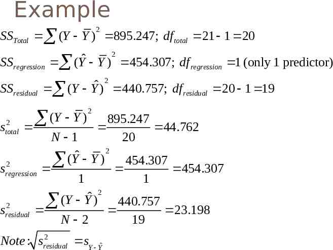
Example 2 69 SSTotal (Y Y ) 895.247; df total 21 1 20 SS regression SS residual 2 total s 2 ˆ (Y Y ) 454.307; df regression 1 (only 1 predictor) 2 ˆ (Y Y ) 440.757; df residual 20 1 19 (Y Y ) 2 895.247 44.762 20 N 1 2 ˆ (Y Y ) 454.307 2 sregression 454.307 1 1 2 ˆ (Y Y ) 440.757 2 sresidual 23.198 N 2 19 2 Note : sresidual sY Yˆ
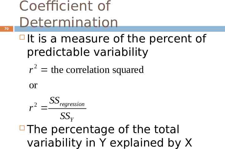
70 Coefficient of Determination It is a measure of the percent of predictable variability r 2 the correlation squared or SS regression 2 r SSY The percentage of the total variability in Y explained by X
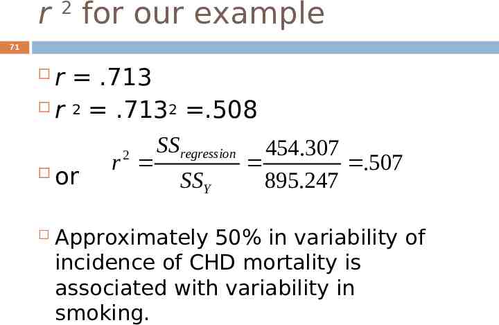
r 2 for our example 71 r .713 r 2 .7132 .508 SS regression 454.307 2 r .507 or SSY 895.247 Approximately 50% in variability of incidence of CHD mortality is associated with variability in smoking.
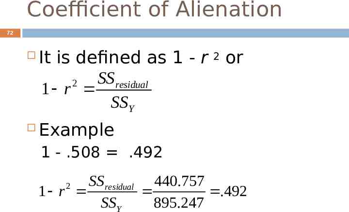
Coefficient of Alienation 72 It is defined as 1 - r SS residual 2 1 r SSY Example 2 or 1 - .508 .492 SS residual 440.757 1 r .492 SSY 895.247 2
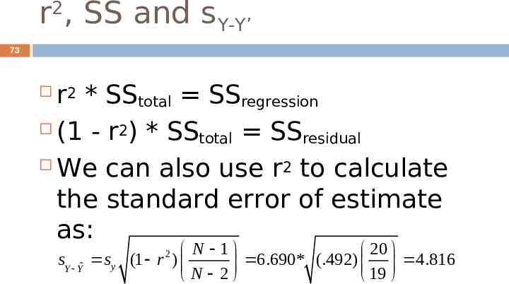
r2, SS and sY-Y’ 73 r * SStotal SSregression (1 - r2) * SS total SSresidual We can also use r2 to calculate the standard error of estimate as: 2 sY Yˆ s y N 1 20 (1 r ) 6.690* (.492) 4.816 N 2 19 2
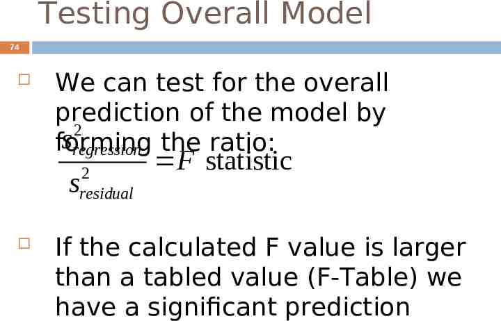
Testing Overall Model 74 We can test for the overall prediction of the model by 2 sregression the ratio: forming 2 residual s F statistic If the calculated F value is larger than a tabled value (F-Table) we have a significant prediction
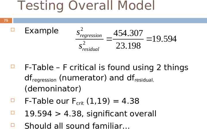
Testing Overall Model 75 Example 2 sregression 2 sresidual 454.307 19.594 23.198 F-Table – F critical is found using 2 things dfregression (numerator) and dfresidual. (demoninator) F-Table our Fcrit (1,19) 4.38 19.594 4.38, significant overall Should all sound familiar
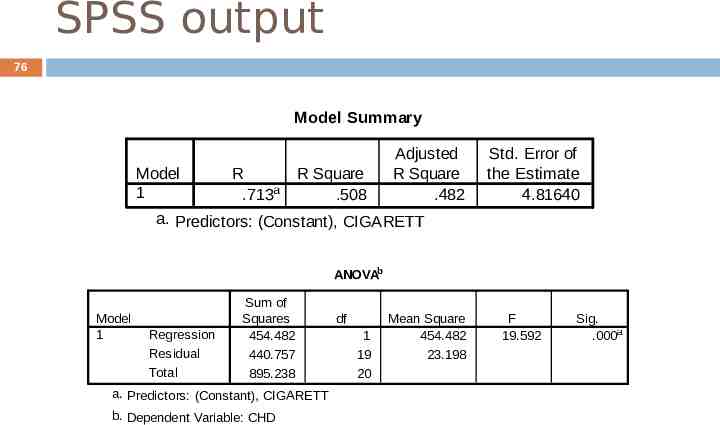
SPSS output 76 Model Summary Model 1 R .713a R Square .508 Adjusted R Square .482 Std. Error of the Estimate 4.81640 a. Predictors: (Constant), CIGARETT ANOVAb Model 1 Regression Residual Total Sum of Squares 454.482 440.757 895.238 a. Predictors: (Constant), CIGARETT b. Dependent Variable: CHD df 1 19 20 Mean Square 454.482 23.198 F 19.592 Sig. .000a
Testing Slope and Intercept 77 The regression coefficients can be tested for significance Each coefficient divided by it’s standard error equals a t value that can also be looked up in a ttable Each coefficient is tested against 0
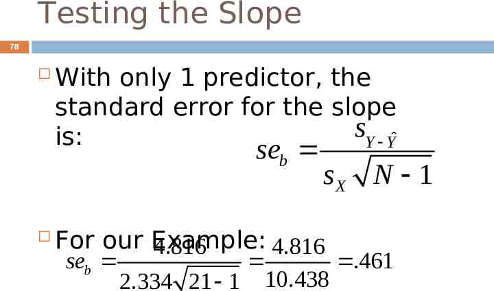
Testing the Slope 78 With only 1 predictor, the standard error for the slope sY Yˆ is: seb sX N 1 For our Example: 4.816 4.816 seb .461 2.334 21 1 10.438
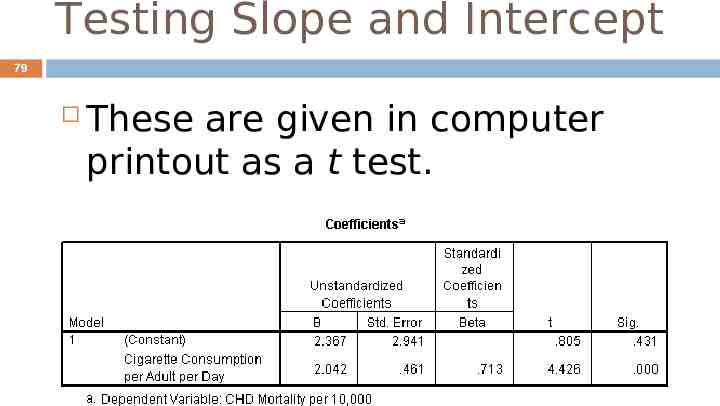
Testing Slope and Intercept 79 These are given in computer printout as a t test.
Testing 80 The t values in the second from right column are tests on slope and intercept. The associated p values are next to them. The slope is significantly different from zero, but not the intercept. Why do we care?
Testing 81 What does it mean if slope is not significant? How does that relate to test on r? What if the intercept is not significant? Does significant slope mean we predict quite well?