Chapter 4: Unsupervised Learning
95 Slides1.04 MB
Chapter 4: Unsupervised Learning
Road map Basic concepts K-means algorithm Representation of clusters Hierarchical clustering Distance functions Data standardization Handling mixed attributes Which clustering algorithm to use? Cluster evaluation Discovering holes and data regions Summary CS583, Bing Liu, UIC 2
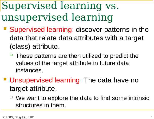
Supervised learning vs. unsupervised learning Supervised learning: discover patterns in the data that relate data attributes with a target (class) attribute. These patterns are then utilized to predict the values of the target attribute in future data instances. Unsupervised learning: The data have no target attribute. We want to explore the data to find some intrinsic structures in them. CS583, Bing Liu, UIC 3
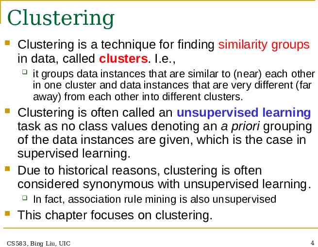
Clustering Clustering is a technique for finding similarity groups in data, called clusters. I.e., Clustering is often called an unsupervised learning task as no class values denoting an a priori grouping of the data instances are given, which is the case in supervised learning. Due to historical reasons, clustering is often considered synonymous with unsupervised learning. it groups data instances that are similar to (near) each other in one cluster and data instances that are very different (far away) from each other into different clusters. In fact, association rule mining is also unsupervised This chapter focuses on clustering. CS583, Bing Liu, UIC 4
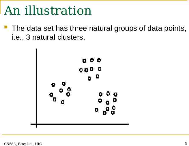
An illustration The data set has three natural groups of data points, i.e., 3 natural clusters. CS583, Bing Liu, UIC 5
What is clustering for? Let us see some real-life examples Example 1: groups people of similar sizes together to make “small”, “medium” and “large” T-Shirts. Tailor-made for each person: too expensive One-size-fits-all: does not fit all. Example 2: In marketing, segment customers according to their similarities To do targeted marketing. CS583, Bing Liu, UIC 6
What is clustering for? (cont ) Example 3: Given a collection of text documents, we want to organize them according to their content similarities, To produce a topic hierarchy In fact, clustering is one of the most utilized data mining techniques. It has a long history, and used in almost every field, e.g., medicine, psychology, botany, sociology, biology, archeology, marketing, insurance, libraries, etc. In recent years, due to the rapid increase of online documents, text clustering becomes important. CS583, Bing Liu, UIC 7
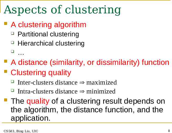
Aspects of clustering A clustering algorithm A distance (similarity, or dissimilarity) function Clustering quality Partitional clustering Hierarchical clustering Inter-clusters distance maximized Intra-clusters distance minimized The quality of a clustering result depends on the algorithm, the distance function, and the application. CS583, Bing Liu, UIC 8
Road map Basic concepts K-means algorithm Representation of clusters Hierarchical clustering Distance functions Data standardization Handling mixed attributes Which clustering algorithm to use? Cluster evaluation Discovering holes and data regions Summary CS583, Bing Liu, UIC 9
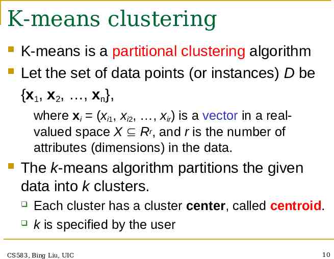
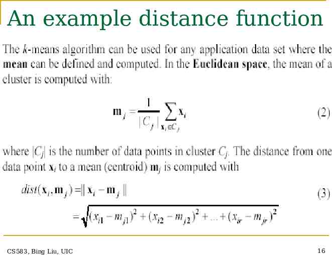
K-means clustering K-means is a partitional clustering algorithm Let the set of data points (or instances) D be {x1, x2, , xn}, where xi (xi1, xi2, , xir) is a vector in a realvalued space X Rr, and r is the number of attributes (dimensions) in the data. The k-means algorithm partitions the given data into k clusters. Each cluster has a cluster center, called centroid. k is specified by the user CS583, Bing Liu, UIC 10
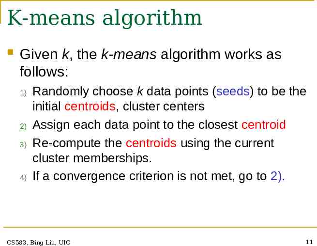
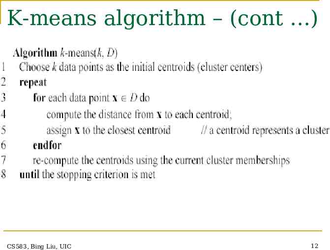
K-means algorithm Given k, the k-means algorithm works as follows: 1) 2) 3) 4) Randomly choose k data points (seeds) to be the initial centroids, cluster centers Assign each data point to the closest centroid Re-compute the centroids using the current cluster memberships. If a convergence criterion is not met, go to 2). CS583, Bing Liu, UIC 11
K-means algorithm – (cont ) CS583, Bing Liu, UIC 12
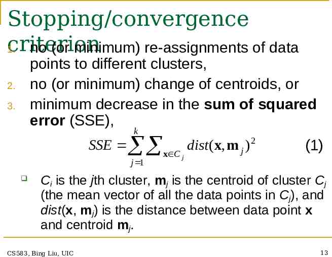
Stopping/convergence criterion 1. no (or minimum) re-assignments of data points to different clusters, no (or minimum) change of centroids, or minimum decrease in the sum of squared error (SSE), 2. 3. k SSE j 1 x C j dist (x, m j ) 2 (1) Ci is the jth cluster, mj is the centroid of cluster Cj (the mean vector of all the data points in Cj), and dist(x, mj) is the distance between data point x and centroid mj. CS583, Bing Liu, UIC 13
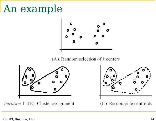
An example CS583, Bing Liu, UIC 14
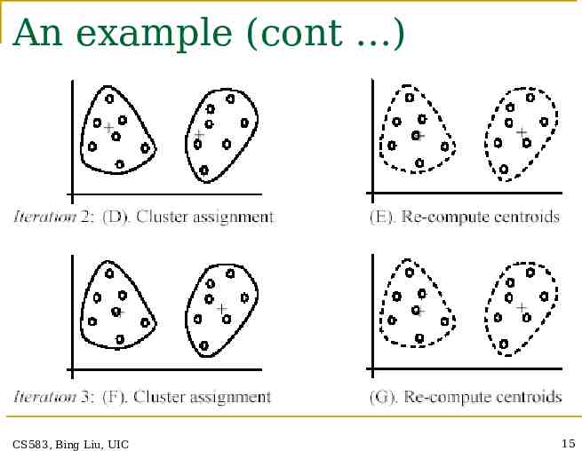
An example (cont ) CS583, Bing Liu, UIC 15
An example distance function CS583, Bing Liu, UIC 16
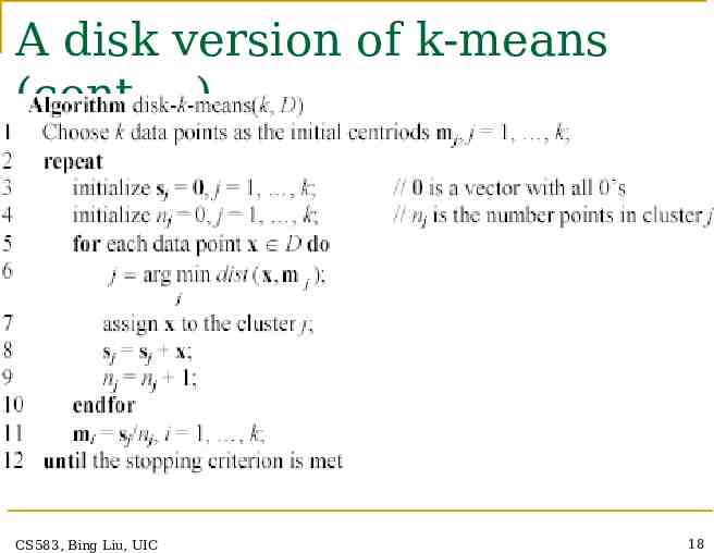
A disk version of k-means K-means can be implemented with data on disk It can be used to cluster large datasets that do not fit in main memory We need to control the number of iterations In each iteration, it scans the data once. as the centroids can be computed incrementally In practice, a limited is set ( 50). Not the best method. There are other scaleup algorithms, e.g., BIRCH. CS583, Bing Liu, UIC 17
A disk version of k-means (cont ) CS583, Bing Liu, UIC 18
Strengths of k-means Strengths: Simple: easy to understand and to implement Efficient: Time complexity: O(tkn), where n is the number of data points, k is the number of clusters, and t is the number of iterations. Since both k and t are small. k-means is considered a linear algorithm. K-means is the most popular clustering algorithm. Note that: it terminates at a local optimum if SSE is used. The global optimum is hard to find due to complexity. CS583, Bing Liu, UIC 19
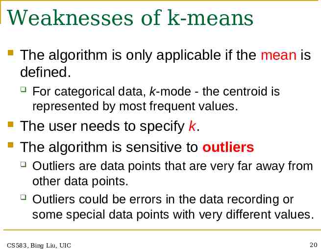
Weaknesses of k-means The algorithm is only applicable if the mean is defined. For categorical data, k-mode - the centroid is represented by most frequent values. The user needs to specify k. The algorithm is sensitive to outliers Outliers are data points that are very far away from other data points. Outliers could be errors in the data recording or some special data points with very different values. CS583, Bing Liu, UIC 20
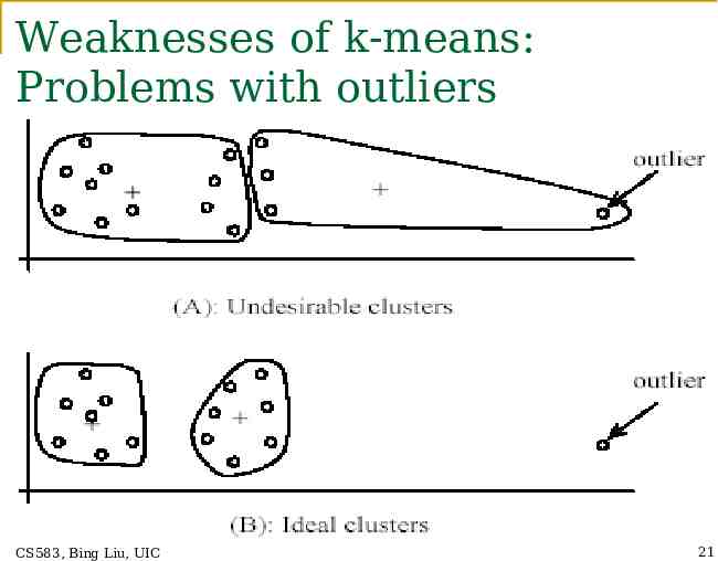
Weaknesses of k-means: Problems with outliers CS583, Bing Liu, UIC 21
Weaknesses of k-means: To deal with outliers One method is to remove some data points in the clustering process that are much further away from the centroids than other data points. To be safe, we may want to monitor these possible outliers over a few iterations and then decide to remove them. Another method is to perform random sampling. Since in sampling we only choose a small subset of the data points, the chance of selecting an outlier is very small. Assign the rest of the data points to the clusters by distance or similarity comparison, or classification CS583, Bing Liu, UIC 22
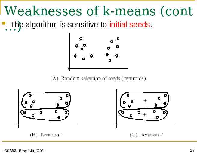
Weaknesses of k-means (cont The algorithm is sensitive to initial seeds. ) CS583, Bing Liu, UIC 23
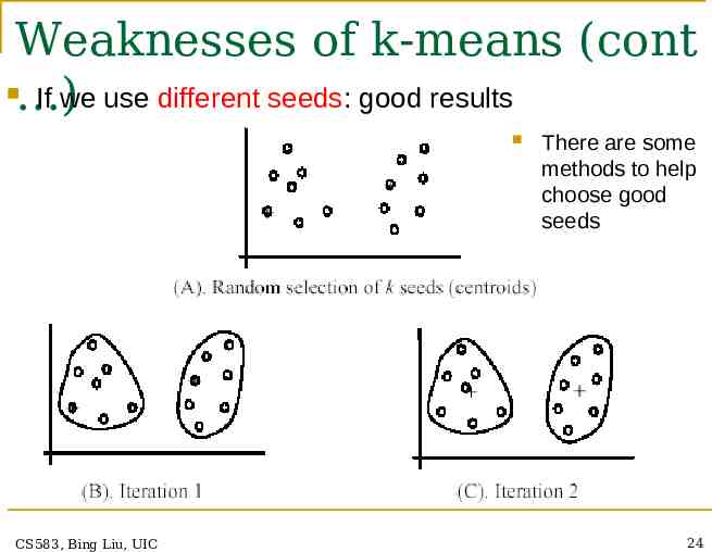
Weaknesses of k-means (cont If we use different seeds: good results ) CS583, Bing Liu, UIC There are some methods to help choose good seeds 24
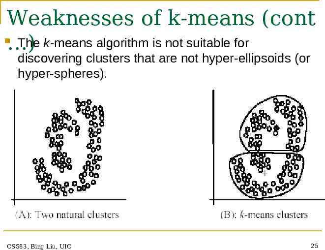
Weaknesses of k-means (cont The k-means algorithm is not suitable for ) discovering clusters that are not hyper-ellipsoids (or hyper-spheres). CS583, Bing Liu, UIC 25
K-means summary Despite weaknesses, k-means is still the most popular algorithm due to its simplicity, efficiency and No clear evidence that any other clustering algorithm performs better in general other clustering algorithms have their own lists of weaknesses. although they may be more suitable for some specific types of data or applications. Comparing different clustering algorithms is a difficult task. No one knows the correct clusters! CS583, Bing Liu, UIC 26
Road map Basic concepts K-means algorithm Representation of clusters Hierarchical clustering Distance functions Data standardization Handling mixed attributes Which clustering algorithm to use? Cluster evaluation Discovering holes and data regions Summary CS583, Bing Liu, UIC 27
Common ways to represent clusters Use the centroid of each cluster to represent the cluster. compute the radius and standard deviation of the cluster to determine its spread in each dimension The centroid representation alone works well if the clusters are of the hyper-spherical shape. If clusters are elongated or are of other shapes, centroids are not sufficient CS583, Bing Liu, UIC 28
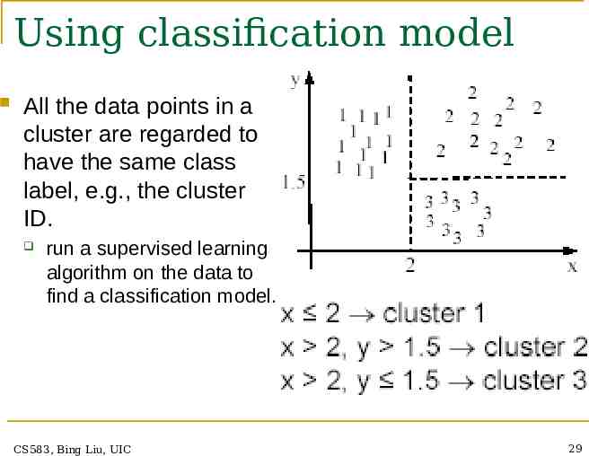
Using classification model All the data points in a cluster are regarded to have the same class label, e.g., the cluster ID. run a supervised learning algorithm on the data to find a classification model. CS583, Bing Liu, UIC 29
Use frequent values to represent cluster This method is mainly for clustering of categorical data (e.g., k-modes clustering). Main method used in text clustering, where a small set of frequent words in each cluster is selected to represent the cluster. CS583, Bing Liu, UIC 30
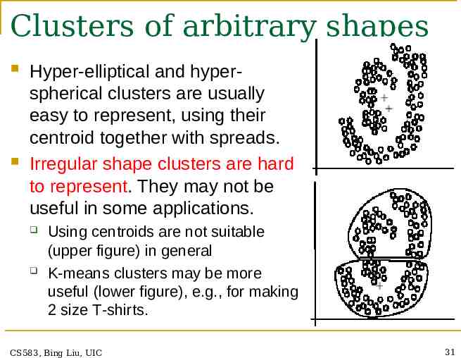
Clusters of arbitrary shapes Hyper-elliptical and hyperspherical clusters are usually easy to represent, using their centroid together with spreads. Irregular shape clusters are hard to represent. They may not be useful in some applications. Using centroids are not suitable (upper figure) in general K-means clusters may be more useful (lower figure), e.g., for making 2 size T-shirts. CS583, Bing Liu, UIC 31
Road map Basic concepts K-means algorithm Representation of clusters Hierarchical clustering Distance functions Data standardization Handling mixed attributes Which clustering algorithm to use? Cluster evaluation Discovering holes and data regions Summary CS583, Bing Liu, UIC 32
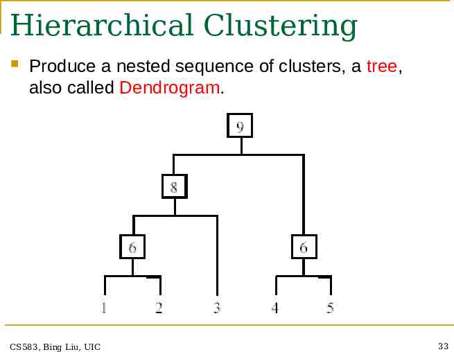
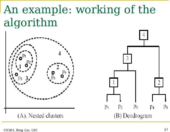
Hierarchical Clustering Produce a nested sequence of clusters, a tree, also called Dendrogram. CS583, Bing Liu, UIC 33
Types of hierarchical clustering Agglomerative (bottom up) clustering: It builds the dendrogram (tree) from the bottom level, and merges the most similar (or nearest) pair of clusters stops when all the data points are merged into a single cluster (i.e., the root cluster). Divisive (top down) clustering: It starts with all data points in one cluster, the root. Splits the root into a set of child clusters. Each child cluster is recursively divided further stops when only singleton clusters of individual data points remain, i.e., each cluster with only a single point CS583, Bing Liu, UIC 34
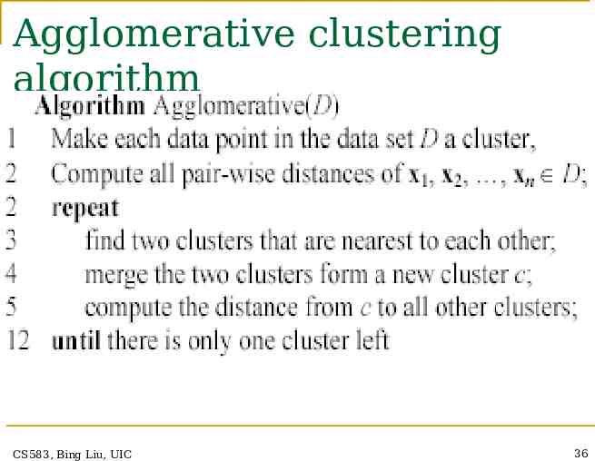
Agglomerative clustering It is more popular then divisive methods. At the beginning, each data point forms a cluster (also called a node). Merge nodes/clusters that have the least distance. Go on merging Eventually all nodes belong to one cluster CS583, Bing Liu, UIC 35
Agglomerative clustering algorithm CS583, Bing Liu, UIC 36
An example: working of the algorithm CS583, Bing Liu, UIC 37
Measuring the distance of two clusters A few ways to measure distances of two clusters. Results in different variations of the algorithm. Single link Complete link Average link Centroids CS583, Bing Liu, UIC 38
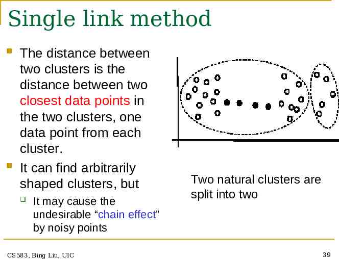
Single link method The distance between two clusters is the distance between two closest data points in the two clusters, one data point from each cluster. It can find arbitrarily shaped clusters, but It may cause the undesirable “chain effect” by noisy points CS583, Bing Liu, UIC Two natural clusters are split into two 39
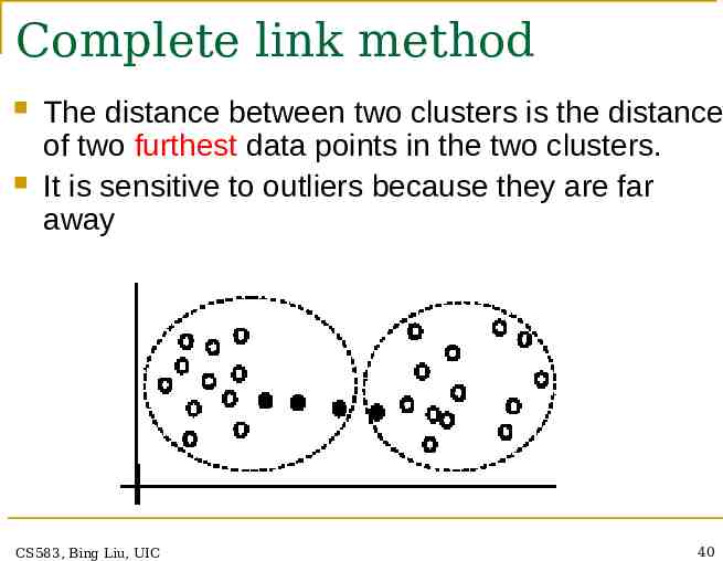
Complete link method The distance between two clusters is the distance of two furthest data points in the two clusters. It is sensitive to outliers because they are far away CS583, Bing Liu, UIC 40
Average link and centroid methods Average link: A compromise between the sensitivity of complete-link clustering to outliers and the tendency of single-link clustering to form long chains that do not correspond to the intuitive notion of clusters as compact, spherical objects. In this method, the distance between two clusters is the average distance of all pair-wise distances between the data points in two clusters. Centroid method: In this method, the distance between two clusters is the distance between their centroids CS583, Bing Liu, UIC 41
The complexity All the algorithms are at least O(n2). n is the number of data points. Single link can be done in O(n2). Complete and average links can be done in O(n2logn). Due the complexity, hard to use for large data sets. Sampling Scale-up methods (e.g., BIRCH). CS583, Bing Liu, UIC 42
Road map Basic concepts K-means algorithm Representation of clusters Hierarchical clustering Distance functions Data standardization Handling mixed attributes Which clustering algorithm to use? Cluster evaluation Discovering holes and data regions Summary CS583, Bing Liu, UIC 43
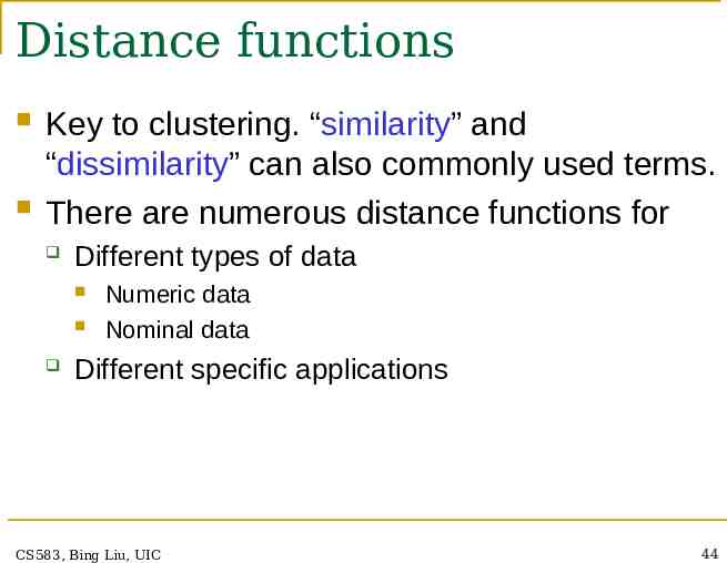
Distance functions Key to clustering. “similarity” and “dissimilarity” can also commonly used terms. There are numerous distance functions for Different types of data Numeric data Nominal data Different specific applications CS583, Bing Liu, UIC 44
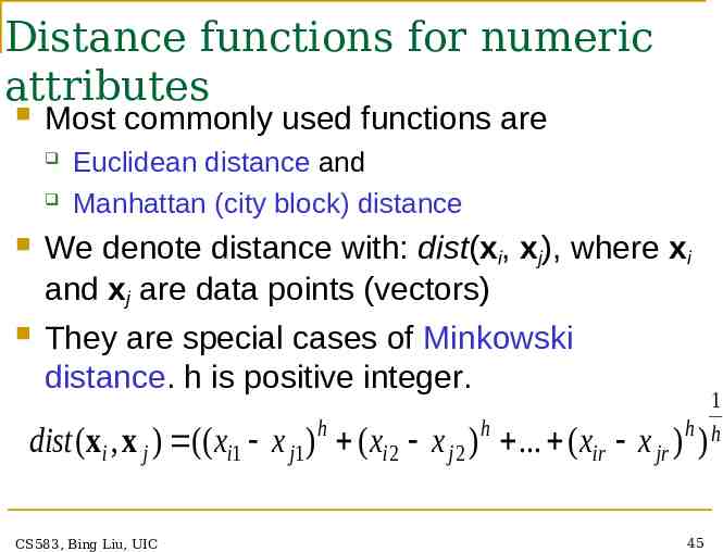
Distance functions for numeric attributes Most commonly used functions are Euclidean distance and Manhattan (city block) distance We denote distance with: dist(xi, xj), where xi and xj are data points (vectors) They are special cases of Minkowski distance. h is positive integer. h h dist (xi , x j ) (( xi1 x j1 ) ( xi 2 x j 2 ) . ( xir x jr CS583, Bing Liu, UIC 1 h h ) ) 45
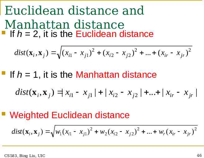
Euclidean distance and Manhattan distance If h 2, it is the Euclidean distance dist (xi , x j ) ( xi1 x j1 ) 2 ( xi 2 x j 2 ) 2 . ( xir x jr ) 2 If h 1, it is the Manhattan distance dist (xi , x j ) xi1 x j1 xi 2 x j 2 . xir x jr Weighted Euclidean distance dist (xi , x j ) w1 ( xi1 x j1 ) 2 w2 ( xi 2 x j 2 ) 2 . wr ( xir x jr ) 2 CS583, Bing Liu, UIC 46
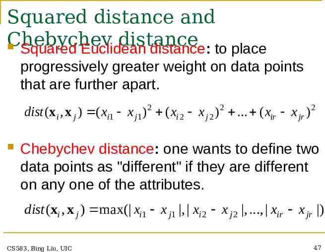
Squared distance and Chebychev distance Squared Euclidean distance: to place progressively greater weight on data points that are further apart. dist (xi , x j ) ( xi1 x j1 ) 2 ( xi 2 x j 2 ) 2 . ( xir x jr ) 2 Chebychev distance: one wants to define two data points as "different" if they are different on any one of the attributes. dist (xi , x j ) max( xi1 x j1 , xi 2 x j 2 , ., xir x jr ) CS583, Bing Liu, UIC 47
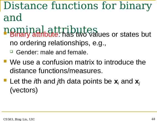
Distance functions for binary and nominal attributes Binary attribute: has two values or states but no ordering relationships, e.g., Gender: male and female. We use a confusion matrix to introduce the distance functions/measures. Let the ith and jth data points be xi and xj (vectors) CS583, Bing Liu, UIC 48
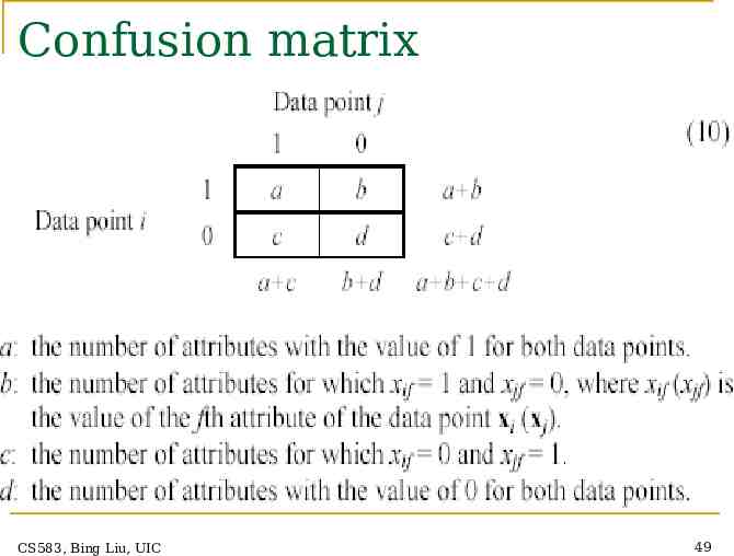
Confusion matrix CS583, Bing Liu, UIC 49
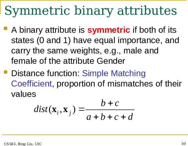
Symmetric binary attributes A binary attribute is symmetric if both of its states (0 and 1) have equal importance, and carry the same weights, e.g., male and female of the attribute Gender Distance function: Simple Matching Coefficient, proportion of mismatches of their values b c dist (xi , x j ) a b c d CS583, Bing Liu, UIC 50
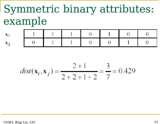
Symmetric binary attributes: example CS583, Bing Liu, UIC 51
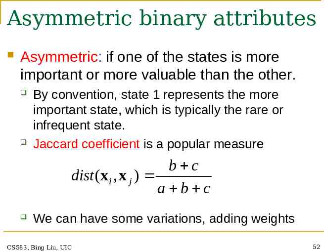
Asymmetric binary attributes Asymmetric: if one of the states is more important or more valuable than the other. By convention, state 1 represents the more important state, which is typically the rare or infrequent state. Jaccard coefficient is a popular measure b c dist (xi , x j ) a b c We can have some variations, adding weights CS583, Bing Liu, UIC 52
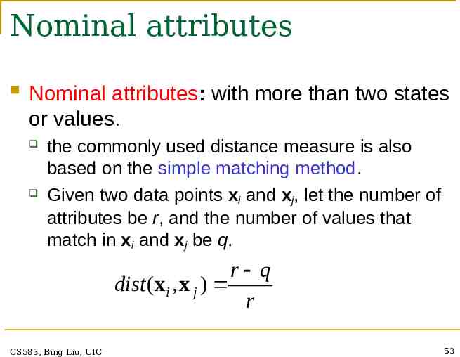
Nominal attributes Nominal attributes: with more than two states or values. the commonly used distance measure is also based on the simple matching method. Given two data points xi and xj, let the number of attributes be r, and the number of values that match in xi and xj be q. r q dist (xi , x j ) r CS583, Bing Liu, UIC 53
Distance function for text A text document consists of a sequence of documents sentences and each sentence consists of a sequence of words. To simplify: a document is usually considered a “bag” of words in document clustering. Sequence and position of words are ignored. A document is represented with a vector just like a normal data point. It is common to use similarity to compare two documents rather than distance. The most commonly used similarity function is the cosine similarity. We will study this later. CS583, Bing Liu, UIC 54
Road map Basic concepts K-means algorithm Representation of clusters Hierarchical clustering Distance functions Data standardization Handling mixed attributes Which clustering algorithm to use? Cluster evaluation Discovering holes and data regions Summary CS583, Bing Liu, UIC 55
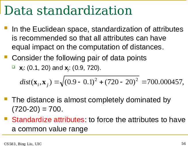
Data standardization In the Euclidean space, standardization of attributes is recommended so that all attributes can have equal impact on the computation of distances. Consider the following pair of data points xi: (0.1, 20) and xj: (0.9, 720). dist (xi , x j ) (0.9 0.1) 2 (720 20) 2 700.000457, The distance is almost completely dominated by (720-20) 700. Standardize attributes: to force the attributes to have a common value range CS583, Bing Liu, UIC 56
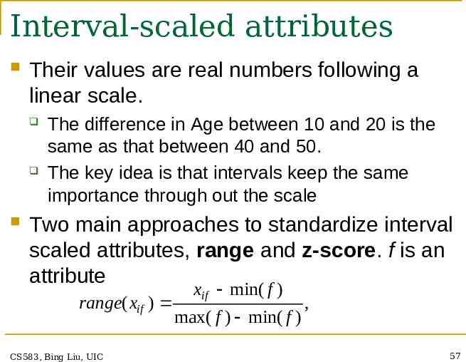
Interval-scaled attributes Their values are real numbers following a linear scale. The difference in Age between 10 and 20 is the same as that between 40 and 50. The key idea is that intervals keep the same importance through out the scale Two main approaches to standardize interval scaled attributes, range and z-score. f is an attribute range( xif ) CS583, Bing Liu, UIC xif min( f ) max( f ) min( f ) , 57
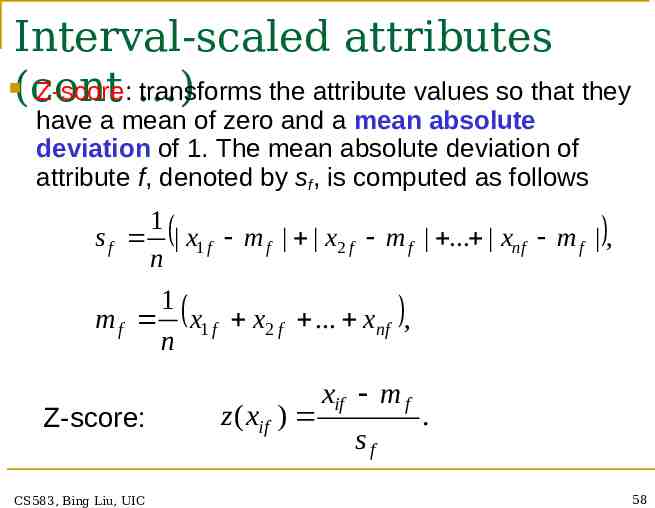
Interval-scaled attributes (cont Z-score: ) transforms the attribute values so that they have a mean of zero and a mean absolute deviation of 1. The mean absolute deviation of attribute f, denoted by sf, is computed as follows 1 s f x1 f m f x2 f m f . xnf m f , n 1 m f x1 f x2 f . xnf , n Z-score: CS583, Bing Liu, UIC z ( xif ) xif m f sf . 58
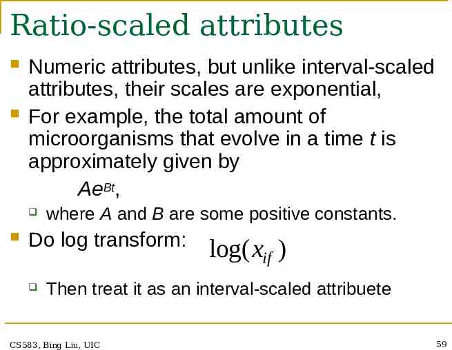
Ratio-scaled attributes Numeric attributes, but unlike interval-scaled attributes, their scales are exponential, For example, the total amount of microorganisms that evolve in a time t is approximately given by AeBt, where A and B are some positive constants. Do log transform: log( xif ) Then treat it as an interval-scaled attribuete CS583, Bing Liu, UIC 59
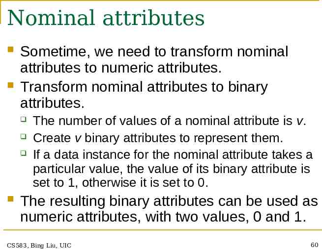
Nominal attributes Sometime, we need to transform nominal attributes to numeric attributes. Transform nominal attributes to binary attributes. The number of values of a nominal attribute is v. Create v binary attributes to represent them. If a data instance for the nominal attribute takes a particular value, the value of its binary attribute is set to 1, otherwise it is set to 0. The resulting binary attributes can be used as numeric attributes, with two values, 0 and 1. CS583, Bing Liu, UIC 60
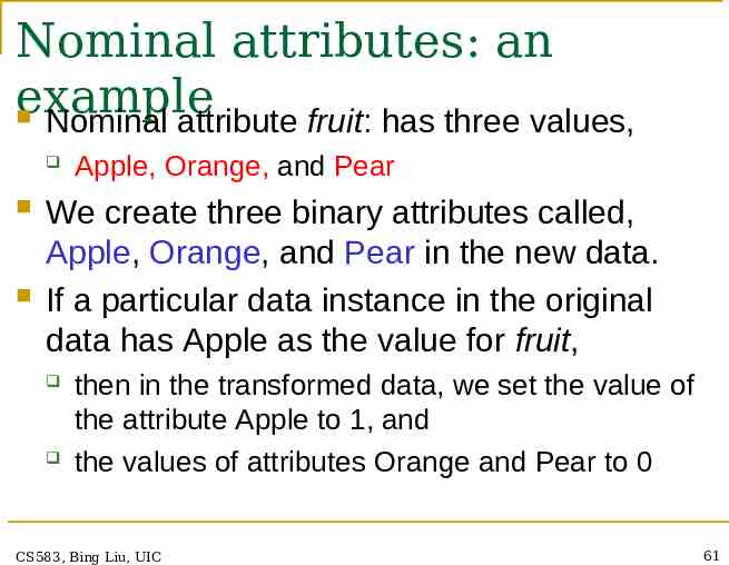
Nominal attributes: an example Nominal attribute fruit: has three values, Apple, Orange, and Pear We create three binary attributes called, Apple, Orange, and Pear in the new data. If a particular data instance in the original data has Apple as the value for fruit, then in the transformed data, we set the value of the attribute Apple to 1, and the values of attributes Orange and Pear to 0 CS583, Bing Liu, UIC 61
Ordinal attributes Ordinal attribute: an ordinal attribute is like a nominal attribute, but its values have a numerical ordering. E.g., Age attribute with values: Young, MiddleAge and Old. They are ordered. Common approach to standardization: treat is as an interval-scaled attribute. CS583, Bing Liu, UIC 62
Road map Basic concepts K-means algorithm Representation of clusters Hierarchical clustering Distance functions Data standardization Handling mixed attributes Which clustering algorithm to use? Cluster evaluation Discovering holes and data regions Summary CS583, Bing Liu, UIC 63
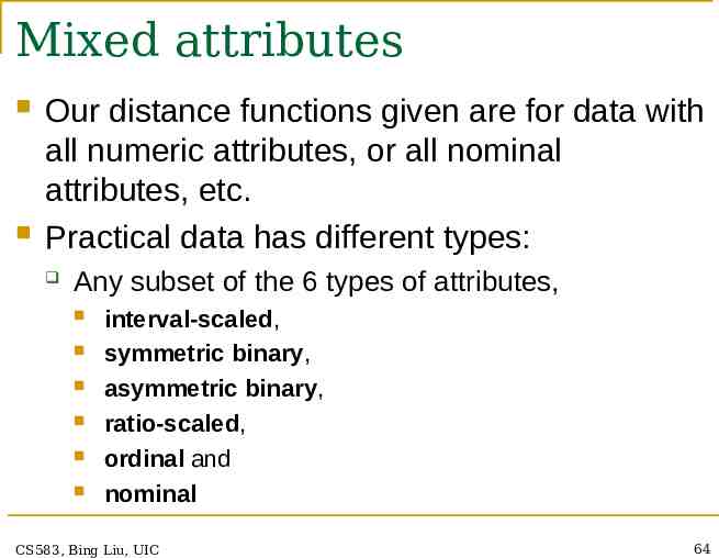
Mixed attributes Our distance functions given are for data with all numeric attributes, or all nominal attributes, etc. Practical data has different types: Any subset of the 6 types of attributes, interval-scaled, symmetric binary, asymmetric binary, ratio-scaled, ordinal and nominal CS583, Bing Liu, UIC 64
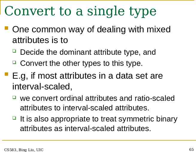
Convert to a single type One common way of dealing with mixed attributes is to Decide the dominant attribute type, and Convert the other types to this type. E.g, if most attributes in a data set are interval-scaled, we convert ordinal attributes and ratio-scaled attributes to interval-scaled attributes. It is also appropriate to treat symmetric binary attributes as interval-scaled attributes. CS583, Bing Liu, UIC 65
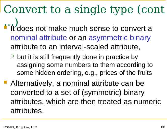
Convert to a single type (cont ) It does not make much sense to convert a nominal attribute or an asymmetric binary attribute to an interval-scaled attribute, but it is still frequently done in practice by assigning some numbers to them according to some hidden ordering, e.g., prices of the fruits Alternatively, a nominal attribute can be converted to a set of (symmetric) binary attributes, which are then treated as numeric attributes. CS583, Bing Liu, UIC 66
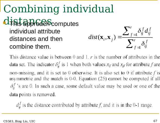
Combining individual distances This approach computes individual attribute distances and then combine them. CS583, Bing Liu, UIC dist (xi , x j ) r f f f 1 ij dij r f f 1 ij 67
Road map Basic concepts K-means algorithm Representation of clusters Hierarchical clustering Distance functions Data standardization Handling mixed attributes Which clustering algorithm to use? Cluster evaluation Discovering holes and data regions Summary CS583, Bing Liu, UIC 68
How to choose a clustering Clustering research has a long history. A vast algorithm collection of algorithms are available. We only introduced several main algorithms. Choosing the “best” algorithm is a challenge. Every algorithm has limitations and works well with certain data distributions. It is very hard, if not impossible, to know what distribution the application data follow. The data may not fully follow any “ideal” structure or distribution required by the algorithms. One also needs to decide how to standardize the data, to choose a suitable distance function and to select other parameter values. CS583, Bing Liu, UIC 69
Choose a clustering algorithm (cont ) Due to these complexities, the common practice is to run several algorithms using different distance functions and parameter settings, and then carefully analyze and compare the results. The interpretation of the results must be based on insight into the meaning of the original data together with knowledge of the algorithms used. Clustering is highly application dependent and to certain extent subjective (personal preferences). CS583, Bing Liu, UIC 70
Road map Basic concepts K-means algorithm Representation of clusters Hierarchical clustering Distance functions Data standardization Handling mixed attributes Which clustering algorithm to use? Cluster evaluation Discovering holes and data regions Summary CS583, Bing Liu, UIC 71
Cluster Evaluation: hard problem The quality of a clustering is very hard to evaluate because We do not know the correct clusters Some methods are used: User inspection Study centroids, and spreads Rules from a decision tree. For text documents, one can read some documents in clusters. CS583, Bing Liu, UIC 72
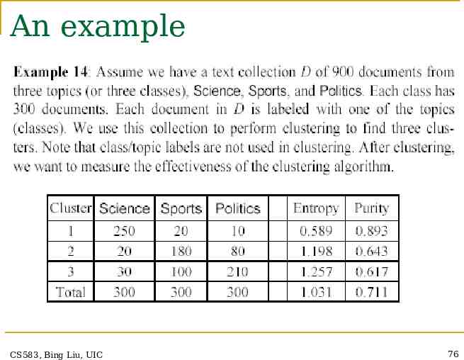
Cluster evaluation: ground truth We use some labeled data (for classification) Assumption: Each class is a cluster. After clustering, a confusion matrix is constructed. From the matrix, we compute various measurements, entropy, purity, precision, recall and F-score. Let the classes in the data D be C (c1, c2, , ck). The clustering method produces k clusters, which divides D into k disjoint subsets, D1, D2, , Dk. CS583, Bing Liu, UIC 73
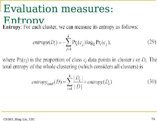
Evaluation measures: Entropy CS583, Bing Liu, UIC 74
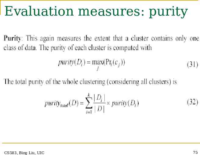
Evaluation measures: purity CS583, Bing Liu, UIC 75
An example CS583, Bing Liu, UIC 76
A remark about ground truth evaluation Commonly used to compare different clustering algorithms. A real-life data set for clustering has no class labels. Thus although an algorithm may perform very well on some labeled data sets, no guarantee that it will perform well on the actual application data at hand. The fact that it performs well on some label data sets does give us some confidence of the quality of the algorithm. This evaluation method is said to be based on external data or information. CS583, Bing Liu, UIC 77
Evaluation based on internal information Intra-cluster cohesion (compactness): Inter-cluster separation (isolation): Cohesion measures how near the data points in a cluster are to the cluster centroid. Sum of squared error (SSE) is a commonly used measure. Separation means that different cluster centroids should be far away from one another. In most applications, expert judgments are still the key. CS583, Bing Liu, UIC 78
Indirect evaluation In some applications, clustering is not the primary task, but used to help perform another task. We can use the performance on the primary task to compare clustering methods. For instance, in an application, the primary task is to provide recommendations on book purchasing to online shoppers. If we can cluster books according to their features, we might be able to provide better recommendations. We can evaluate different clustering algorithms based on how well they help with the recommendation task. Here, we assume that the recommendation can be reliably evaluated. CS583, Bing Liu, UIC 79
Road map Basic concepts K-means algorithm Representation of clusters Hierarchical clustering Distance functions Data standardization Handling mixed attributes Which clustering algorithm to use? Cluster evaluation Discovering holes and data regions Summary CS583, Bing Liu, UIC 80
Holes in data space All the clustering algorithms only group data. Clusters only represent one aspect of the knowledge in the data. Another aspect that we have not studied is the holes. A hole is a region in the data space that contains no or few data points. Reasons: insufficient data in certain areas, and/or certain attribute-value combinations are not possible or seldom occur. CS583, Bing Liu, UIC 81
Holes are useful too Although clusters are important, holes in the space can be quite useful too. For example, in a disease database we may find that certain symptoms and/or test values do not occur together, or when a certain medicine is used, some test values never go beyond certain ranges. Discovery of such information can be important in medical domains because it could mean the discovery of a cure to a disease or some biological laws. CS583, Bing Liu, UIC 82
Data regions and empty regions Given a data space, separate data regions (clusters) and empty regions (holes, with few or no data points). Use a supervised learning technique, i.e., decision tree induction, to separate the two types of regions. Due to the use of a supervised learning method for an unsupervised learning task, an interesting connection is made between the two types of learning paradigms. CS583, Bing Liu, UIC 83
Supervised learning for unsupervised learning Decision tree algorithm is not directly applicable. The problem can be dealt with by a simple idea. it needs at least two classes of data. A clustering data set has no class label for each data point. Regard each point in the data set to have a class label Y. Assume that the data space is uniformly distributed with another type of points, called non-existing points. We give them the class, N. With the N points added, the problem of partitioning the data space into data and empty regions becomes a supervised classification problem. CS583, Bing Liu, UIC 84
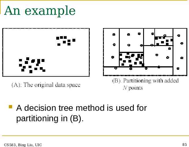
An example A decision tree method is used for partitioning in (B). CS583, Bing Liu, UIC 85
Can it done without adding N points? Yes. Physically adding N points increases the size of the data and thus the running time. More importantly: it is unlikely that we can have points truly uniformly distributed in a high dimensional space as we would need an exponential number of points. Fortunately, no need to physically add any N points. We can compute them when needed CS583, Bing Liu, UIC 86
Characteristics of the It provides representations of the resulting data and approach empty regions in terms of hyper-rectangles, or rules. It detects outliers automatically. Outliers are data points in an empty region. It may not use all attributes in the data just as in a normal decision tree for supervised learning. It can automatically determine what attributes are useful. Subspace clustering Drawback: data regions of irregular shapes are hard to handle since decision tree learning only generates hyper-rectangles (formed by axis-parallel hyperplanes), which are rules. CS583, Bing Liu, UIC 87
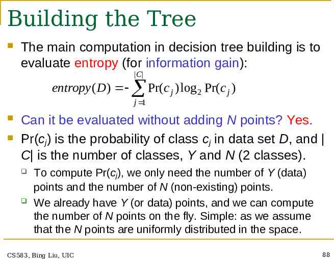
Building the Tree The main computation in decision tree building is to evaluate entropy (for information gain): C entropy ( D) Pr(c ) log j 2 Pr(c j ) j 1 Can it be evaluated without adding N points? Yes. Pr(cj) is the probability of class cj in data set D, and C is the number of classes, Y and N (2 classes). To compute Pr(cj), we only need the number of Y (data) points and the number of N (non-existing) points. We already have Y (or data) points, and we can compute the number of N points on the fly. Simple: as we assume that the N points are uniformly distributed in the space. CS583, Bing Liu, UIC 88
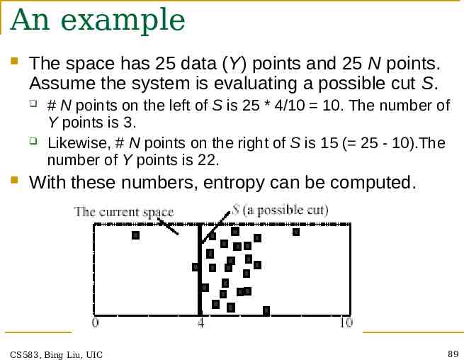
An example The space has 25 data (Y) points and 25 N points. Assume the system is evaluating a possible cut S. # N points on the left of S is 25 * 4/10 10. The number of Y points is 3. Likewise, # N points on the right of S is 15 ( 25 - 10).The number of Y points is 22. With these numbers, entropy can be computed. CS583, Bing Liu, UIC 89
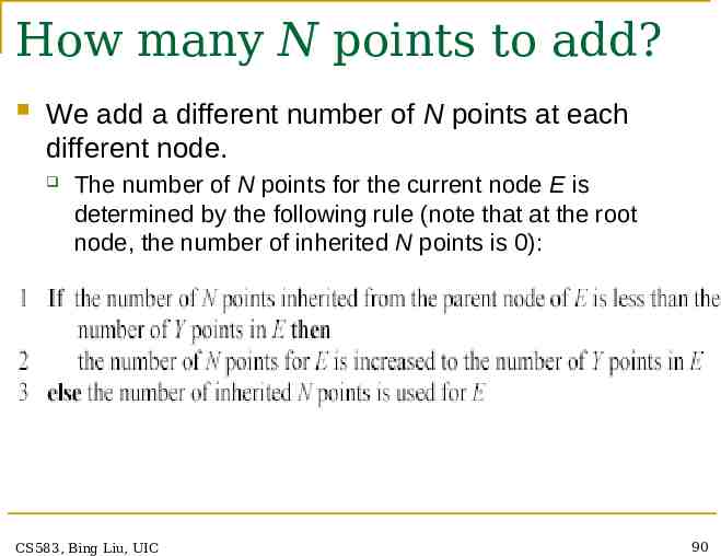
How many N points to add? We add a different number of N points at each different node. The number of N points for the current node E is determined by the following rule (note that at the root node, the number of inherited N points is 0): CS583, Bing Liu, UIC 90
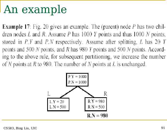
An example CS583, Bing Liu, UIC 91
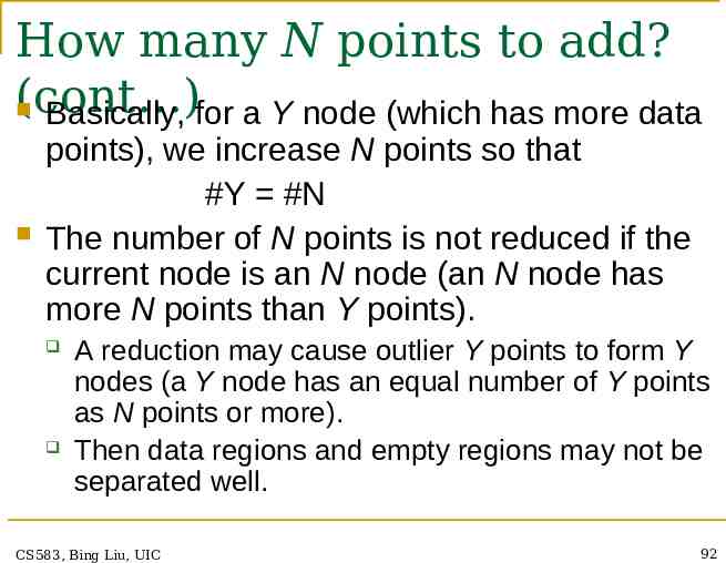
How many N points to add? (cont ) Basically, for a Y node (which has more data points), we increase N points so that #Y #N The number of N points is not reduced if the current node is an N node (an N node has more N points than Y points). A reduction may cause outlier Y points to form Y nodes (a Y node has an equal number of Y points as N points or more). Then data regions and empty regions may not be separated well. CS583, Bing Liu, UIC 92
Building the decision tree Using the above ideas, a decision tree can be built to separate data regions and empty regions. The actual method is more sophisticated as a few other tricky issues need to be handled in tree building and tree pruning. CS583, Bing Liu, UIC 93
Road map Basic concepts K-means algorithm Representation of clusters Hierarchical clustering Distance functions Data standardization Handling mixed attributes Which clustering algorithm to use? Cluster evaluation Discovering holes and data regions Summary CS583, Bing Liu, UIC 94
Summary Clustering is has along history and still active We only introduced several main algorithms. There are many others, e.g., There are a huge number of clustering algorithms More are still coming every year. density based algorithm, sub-space clustering, scale-up methods, neural networks based methods, fuzzy clustering, co-clustering, etc. Clustering is hard to evaluate, but very useful in practice. This partially explains why there are still a large number of clustering algorithms being devised every year. Clustering is highly application dependent and to some extent subjective. CS583, Bing Liu, UIC 95