Chapter 4 Classification and Scoring UIC – CS 594 B. Liu 1

47 Slides305.50 KB
Chapter 4 Classification and Scoring UIC - CS 594 B. Liu 1
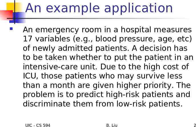
An example application An emergency room in a hospital measures 17 variables (e.g., blood pressure, age, etc) of newly admitted patients. A decision has to be taken whether to put the patient in an intensive-care unit. Due to the high cost of ICU, those patients who may survive less than a month are given higher priority. The problem is to predict high-risk patients and discriminate them from low-risk patients. UIC - CS 594 B. Liu 2
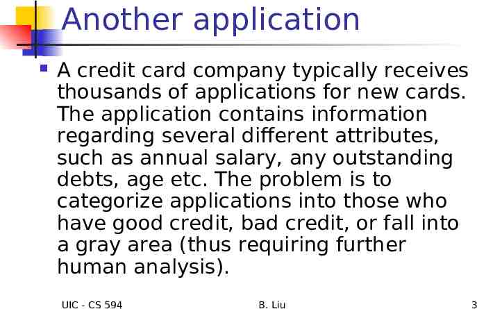
Another application A credit card company typically receives thousands of applications for new cards. The application contains information regarding several different attributes, such as annual salary, any outstanding debts, age etc. The problem is to categorize applications into those who have good credit, bad credit, or fall into a gray area (thus requiring further human analysis). UIC - CS 594 B. Liu 3
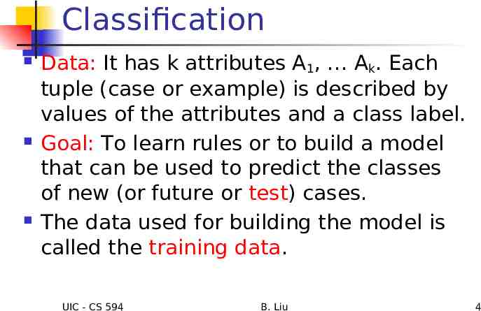
Classification Data: It has k attributes A1, Ak. Each tuple (case or example) is described by values of the attributes and a class label. Goal: To learn rules or to build a model that can be used to predict the classes of new (or future or test) cases. The data used for building the model is called the training data. UIC - CS 594 B. Liu 4
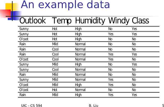
An example data Outlook Temp Humidity Windy Class Sunny Sunny O’cast Rain Rain Rain O’cast Sunny Sunny Rain Sunny O’cast O’cast Rain UIC - CS 594 Hot Hot Hot Mild Cool Cool Cool Mild Cool Mild Mild Mild Hot Mild High High High Normal Normal Normal Normal High Normal Normal Normal High Normal High No Yes No No No Yes Yes No No No Yes Yes No Yes B. Liu Yes Yes No No No Yes No Yes No No No No No Yes 5
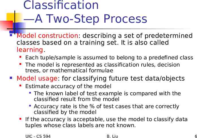
Classification —A Two-Step Process Model construction: describing a set of predetermined classes based on a training set. It is also called learning. Each tuple/sample is assumed to belong to a predefined class The model is represented as classification rules, decision trees, or mathematical formulae Model usage: for classifying future test data/objects Estimate accuracy of the model The known label of test example is compared with the classified result from the model Accuracy rate is the % of test cases that are correctly classified by the model If the accuracy is acceptable, use the model to classify data tuples whose class labels are not known. UIC - CS 594 B. Liu 6
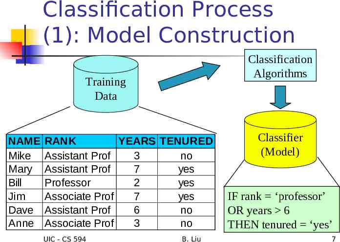
Classification Process (1): Model Construction Classification Algorithms Training Data NAME Mike Mary Bill Jim Dave Anne RANK YEARS TENURED Assistant Prof 3 no Assistant Prof 7 yes Professor 2 yes Associate Prof 7 yes Assistant Prof 6 no Associate Prof 3 no UIC - CS 594 B. Liu Classifier (Model) IF rank ‘professor’ OR years 6 THEN tenured ‘yes’ 7
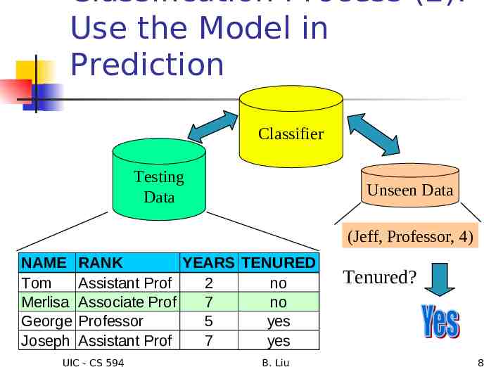
Classification Process (2): Use the Model in Prediction Classifier Testing Data Unseen Data (Jeff, Professor, 4) NAME Tom Merlisa George Joseph RANK YEARS TENURED Assistant Prof 2 no Associate Prof 7 no Professor 5 yes Assistant Prof 7 yes UIC - CS 594 B. Liu Tenured? 8
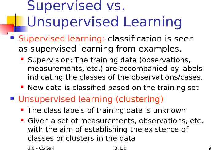
Supervised vs. Unsupervised Learning Supervised learning: classification is seen as supervised learning from examples. Supervision: The training data (observations, measurements, etc.) are accompanied by labels indicating the classes of the observations/cases. New data is classified based on the training set Unsupervised learning (clustering) The class labels of training data is unknown Given a set of measurements, observations, etc. with the aim of establishing the existence of classes or clusters in the data UIC - CS 594 B. Liu 9
Evaluating Classification Methods Predictive accuracy Speed and scalability Robustness: handling noise and missing values Scalability: efficiency in disk-resident databases Interpretability: time to construct the model time to use the model understandable and insight provided by the model Compactness of the model: size of the tree, or the number of rules. UIC - CS 594 B. Liu 10
Different classification techniques There are many techniques for classification Decision trees Naïve Bayesian classifiers Using association rules Neural networks Logistic regression and many more . UIC - CS 594 B. Liu 11
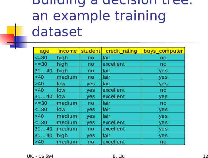
Building a decision tree: an example training dataset age 30 30 31 40 40 40 40 31 40 30 30 40 30 31 40 31 40 40 UIC - CS 594 income student credit rating high no fair high no excellent high no fair medium no fair low yes fair low yes excellent low yes excellent medium no fair low yes fair medium yes fair medium yes excellent medium no excellent high yes fair medium no excellent B. Liu buys computer no no yes yes yes no yes no yes yes yes yes yes no 12
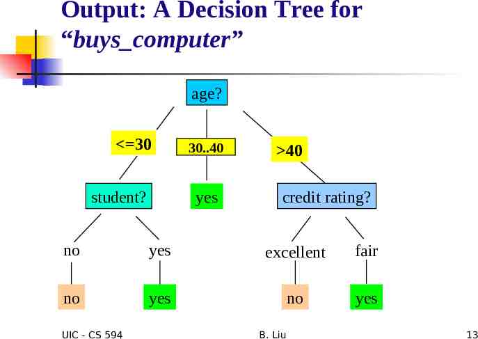
Output: A Decision Tree for “buys computer” age? 30 student? 30.40 overcast yes 40 credit rating? no yes excellent fair no yes no yes UIC - CS 594 B. Liu 13
Inducing a decision tree There are many possible trees How to find the most compact one let’s try it on a credit data that is consistent with the data? Why the most compact? Occam’s razor principle UIC - CS 594 B. Liu 14
Algorithm for Decision Tree Induction Basic algorithm (a greedy algorithm) Tree is constructed in a top-down recursive manner At start, all the training examples are at the root Attributes are categorical (we will talk about continuous-valued attributes later) Examples are partitioned recursively based on selected attributes Test attributes are selected on the basis of a heuristic or statistical measure (e.g., information gain) Conditions for stopping partitioning All exmples for a given node belong to the same class There are no remaining attributes for further partitioning – majority voting is employed for classifying the leaf There are no exmples left UIC - CS 594 B. Liu 15
Building a compact tree The key to building a decision tree which attribute to choose in order to branch. The heuristic is to choose the attribute with the maximum Information Gain based on information theory. Another explanation is to reduce uncertainty as much as possible. UIC - CS 594 B. Liu 16
Information theory Information theory provides a mathematical basis for measuring the information content. To understand the notion of information, think about it as providing the answer to a question, for example, whether a coin will come up heads. If one already has a good guess about the answer, then the actual answer is less informative. If one already knows that the coin is rigged so that it will come with heads with probability 0.99, then a message (advanced information) about the actual outcome of a flip is worth less than it would be for a honest coin. UIC - CS 594 B. Liu 17
Information theory (cont ) For a fair (honest) coin, you have no information, and you are willing to pay more (say in terms of ) for advanced information - less you know, the more valuable the information. Information theory uses this same intuition, but instead of measuring the value for information in dollars, it measures information contents in bits. One bit of information is enough to answer a yes/no question about which one has no idea, such as the flip of a fair coin UIC - CS 594 B. Liu 18
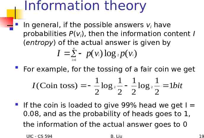
Information theory In general, if the possible answers vi have probabilities P(vi), then the information content I (entropy) of the actual answer is given by n I p(v ) log p(v ) i 2 i i 1 For example, for the tossing of a fair coin we get 1 1 1 1 I (Coin toss) log log 1bit 2 2 2 2 2 2 If the coin is loaded to give 99% head we get I 0.08, and as the probability of heads goes to 1, the information of the actual answer goes to 0 UIC - CS 594 B. Liu 19
Back to decision tree learning For a given example, what is the correct classification? We may think of a decision tree as conveying information about the classification of examples in the table (of examples); The entropy measure characterizes the (im)purity of an arbitrary collection of examples. UIC - CS 594 B. Liu 20
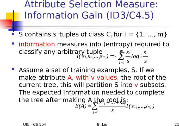
Attribute Selection Measure: Information Gain (ID3/C4.5) S contains si tuples of class Ci for i {1, , m} information measures info (entropy) required to m classify any arbitrary tuple si si I( s1,s2,.,sm ) log 2 s i 1 s Assume a set of training examples, S. If we make attribute A, with v values, the root of the current tree, this will partition S into v subsets. The expected information needed to complete v the tree after making A the root s1 j . sis: mj E(A) j 1 UIC - CS 594 B. Liu s I ( s1 j ,., smj ) 21
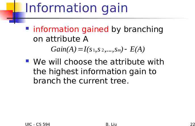
Information gain information gained by branching on attribute A Gain(A) I(s 1, s 2 ,., sm) E(A) We will choose the attribute with the highest information gain to branch the current tree. UIC - CS 594 B. Liu 22
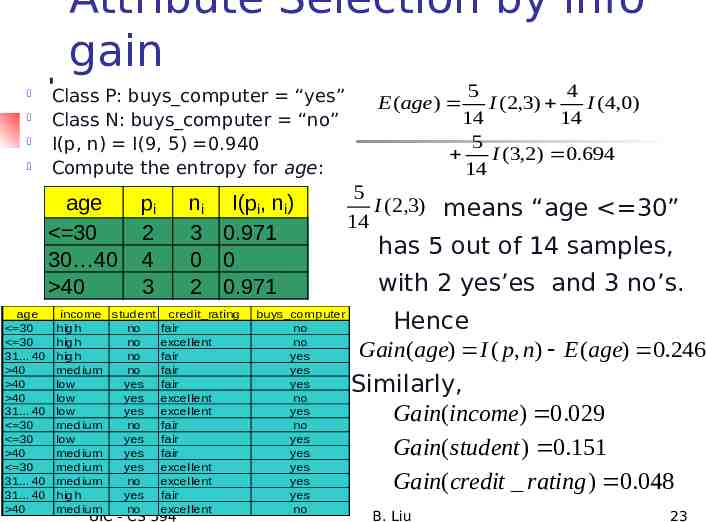
Attribute Selection by info gain Class P: buys computer “yes” Class N: buys computer “no” I(p, n) I(9, 5) 0.940 Compute the entropy for age: age 30 30 40 40 age 30 30 31 40 40 40 40 31 40 30 30 40 30 31 40 31 40 40 pi 2 4 3 ni I(pi, ni) 3 0.971 0 0 2 0.971 income student credit rating high no fair high no excellent high no fair medium no fair low yes fair low yes excellent low yes excellent medium no fair low yes fair medium yes fair medium yes excellent medium no excellent high yes fair medium no excellent UIC - CS 594 buys computer no no yes yes yes no yes no yes yes yes yes yes no 5 4 E ( age) I ( 2,3) I (4,0) 14 14 5 I (3,2) 0.694 14 5 I (2,3) means “age 30” 14 has 5 out of 14 samples, with 2 yes’es and 3 no’s. Hence Gain(age) I ( p, n) E (age) 0.246 Similarly, Gain(income) 0.029 Gain( student ) 0.151 Gain(credit rating ) 0.048 B. Liu 23
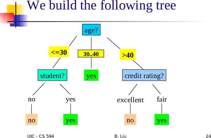
We build the following tree age? 30 student? 30.40 overcast yes 40 credit rating? no yes excellent fair no yes no yes UIC - CS 594 B. Liu 24
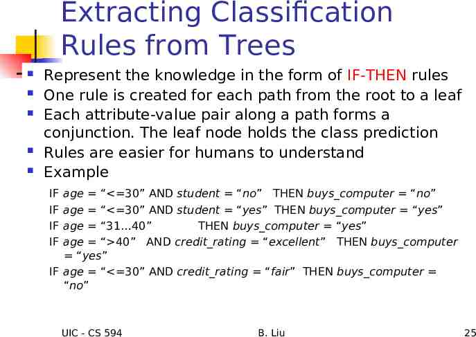
Extracting Classification Rules from Trees Represent the knowledge in the form of IF-THEN rules One rule is created for each path from the root to a leaf Each attribute-value pair along a path forms a conjunction. The leaf node holds the class prediction Rules are easier for humans to understand Example IF IF IF IF age “ 30” AND student “no” THEN buys computer “no” age “ 30” AND student “yes” THEN buys computer “yes” age “31 40” THEN buys computer “yes” age “ 40” AND credit rating “excellent” THEN buys computer “yes” IF age “ 30” AND credit rating “fair” THEN buys computer “no” UIC - CS 594 B. Liu 25
Avoid Overfitting in Classification Overfitting: An tree may overfit the training data Good accuracy on training data but poor on test exmples Too many branches, some may reflect anomalies due to noise or outliers Two approaches to avoid overfitting Prepruning: Halt tree construction early Difficult to decide Postpruning: Remove branches from a “fully grown” tree—get a sequence of progressively pruned trees. This method is commonly used (based on validation set or statistical estimate or MDL) UIC - CS 594 B. Liu 26
Enhancements to basic decision tree induction Allow for continuous-valued attributes Handle missing attribute values Dynamically define new discrete-valued attributes that partition the continuous attribute value into a discrete set of intervals Assign the most common value of the attribute Assign probability to each of the possible values Attribute construction Create new attributes based on existing ones that are sparsely represented. This reduces fragmentation, repetition, and replication UIC - CS 594 B. Liu 27
Bayesian Classification: Why? Probabilistic learning: Classification learning can also be seen as computing P(C c d), i.e., given a data tuple d, what is the probability that d is of class c. (C is the class attribute). How? UIC - CS 594 B. Liu 28
Naïve Bayesian Classifier Let A1 through Ak be attributes with discrete values. They are used to predict a discrete class C. Given an example with observed attribute values a1 through ak. The prediction is the class c such that P(C c A1 a1 . Ak ak) is maximal. UIC - CS 594 B. Liu 29
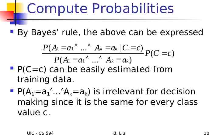
Compute Probabilities By Bayes’ rule, the above can be expressed P( A1 a1 . Ak ak C c) P (C c) P( A1 a1 . Ak ak ) P(C c) can be easily estimated from training data. P(A1 a1 . Ak ak) is irrelevant for decision making since it is the same for every class value c. UIC - CS 594 B. Liu 30
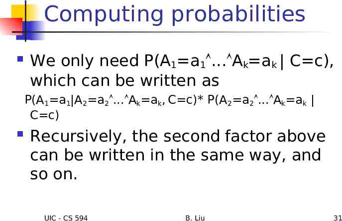
Computing probabilities We only need P(A1 a1 . Ak ak C c), which can be written as P(A1 a1 A2 a2 . Ak ak, C c)* P(A2 a2 . Ak ak C c) Recursively, the second factor above can be written in the same way, and so on. UIC - CS 594 B. Liu 31
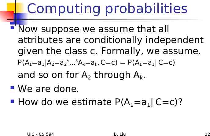
Computing probabilities Now suppose we assume that all attributes are conditionally independent given the class c. Formally, we assume. P(A1 a1 A2 a2 . Ak ak, C c) P(A1 a1 C c) and so on for A2 through Ak. We are done. How do we estimate P(A1 a1 C c)? UIC - CS 594 B. Liu 32
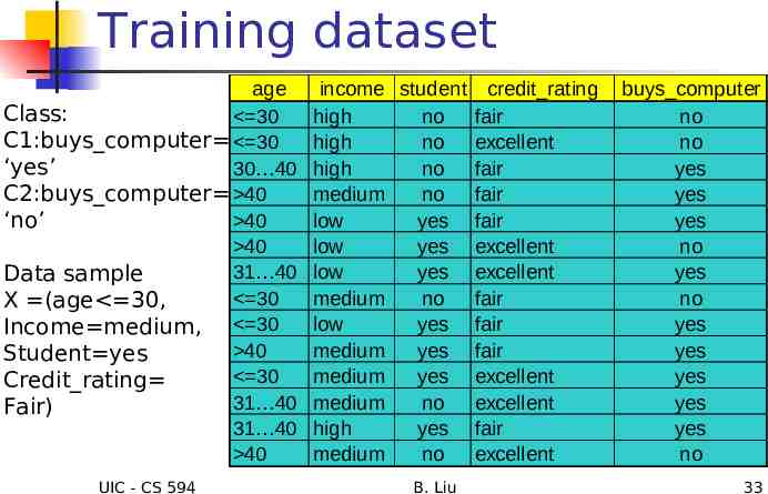
Training dataset age Class: 30 C1:buys computer 30 ‘yes’ 30 40 C2:buys computer 40 40 ‘no’ 40 31 40 Data sample 30 X (age 30, Income medium, 30 40 Student yes 30 Credit rating 31 40 Fair) 31 40 40 UIC - CS 594 income student credit rating high no fair high no excellent high no fair medium no fair low yes fair low yes excellent low yes excellent medium no fair low yes fair medium yes fair medium yes excellent medium no excellent high yes fair medium no excellent B. Liu buys computer no no yes yes yes no yes no yes yes yes yes yes no 33
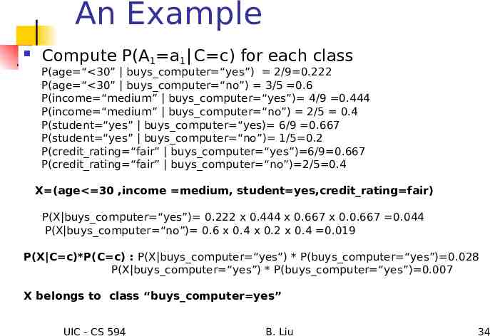
An Example Compute P(A1 a1 C c) for each class P(age “ 30” buys computer “yes”) 2/9 0.222 P(age “ 30” buys computer “no”) 3/5 0.6 P(income “medium” buys computer “yes”) 4/9 0.444 P(income “medium” buys computer “no”) 2/5 0.4 P(student “yes” buys computer “yes) 6/9 0.667 P(student “yes” buys computer “no”) 1/5 0.2 P(credit rating “fair” buys computer “yes”) 6/9 0.667 P(credit rating “fair” buys computer “no”) 2/5 0.4 X (age 30 ,income medium, student yes,credit rating fair) P(X buys computer “yes”) 0.222 x 0.444 x 0.667 x 0.0.667 0.044 P(X buys computer “no”) 0.6 x 0.4 x 0.2 x 0.4 0.019 P(X C c)*P(C c) : P(X buys computer “yes”) * P(buys computer “yes”) 0.028 P(X buys computer “yes”) * P(buys computer “yes”) 0.007 X belongs to class “buys computer yes” UIC - CS 594 B. Liu 34
On Naïve Bayesian Classifier Advantages : Disadvantages Easy to implement Good results obtained in many applications Assumption: class conditional independence, therefore loss of accuracy when the assumption is not true. Practically, dependencies exist How to deal with these dependencies? Bayesian Belief Networks UIC - CS 594 B. Liu 35
Use of Association Rules: Classification Classification: mine a small set of rules existing in the data to form a classifier or predictor. It has a target attribute (on the right side): Class attribute Association: has no fixed target, but we can fix a target. UIC - CS 594 B. Liu 36
Class Association Rules (CARs) Mining rules with a fixed target Right-hand-side of the rules are fixed to a single attribute, which can have a number of values E.g., X a, Y d Class yes X b Class no Call such rules: class association rules UIC - CS 594 B. Liu 37
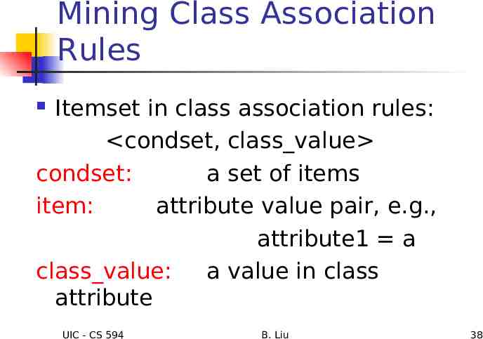
Mining Class Association Rules Itemset in class association rules: condset, class value condset: a set of items item: attribute value pair, e.g., attribute1 a class value: a value in class attribute UIC - CS 594 B. Liu 38
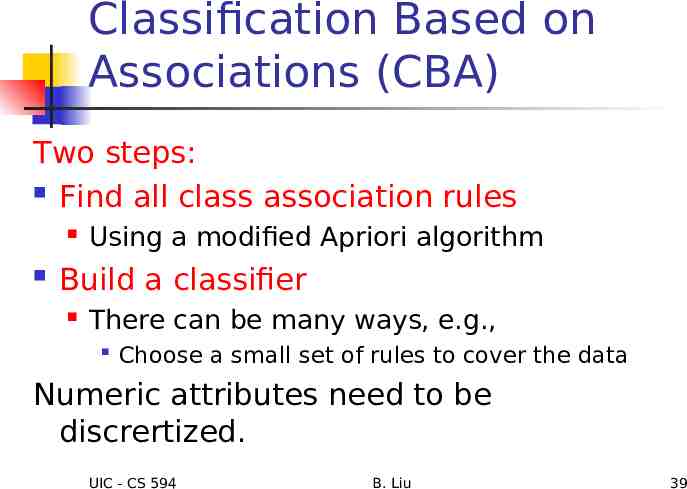
Classification Based on Associations (CBA) Two steps: Find all class association rules Using a modified Apriori algorithm Build a classifier There can be many ways, e.g., Choose a small set of rules to cover the data Numeric attributes need to be discrertized. UIC - CS 594 B. Liu 39
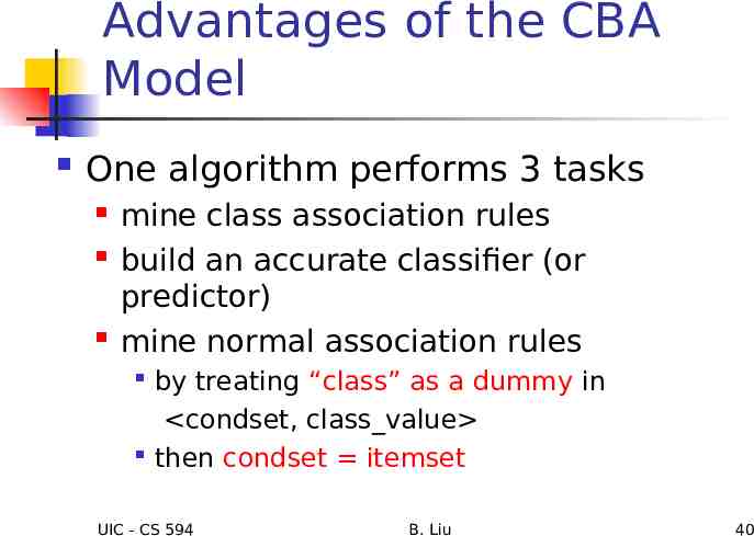
Advantages of the CBA Model One algorithm performs 3 tasks mine class association rules build an accurate classifier (or predictor) mine normal association rules by treating “class” as a dummy in condset, class value then condset itemset UIC - CS 594 B. Liu 40
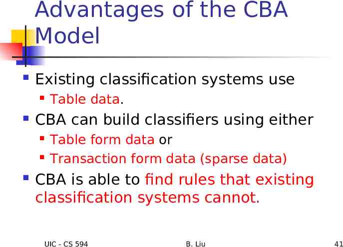
Advantages of the CBA Model Existing classification systems use CBA can build classifiers using either Table data. Table form data or Transaction form data (sparse data) CBA is able to find rules that existing classification systems cannot. UIC - CS 594 B. Liu 41
Assoc. Rules can be Used in Many Ways for Prediction We have so many rules: Select a subset of rules Using Baysian Probability together with the rules Using rule combinations A number of systems have been designed and implemented. UIC - CS 594 B. Liu 42
Other classification techniques Support vector machines Logistic regression K-nearest neighbor Neural networks Genetic algorithms Etc. UIC - CS 594 B. Liu 43
Classification Accuracy or Error Rates Partition: Training-and-testing used for data set with large number of exmples Cross-validation use two independent data sets, e.g., training set (2/3), test set(1/3) divide the data set into k subsamples use k-1 subsamples as training data and one sub-sample as test data—k-fold cross-validation for data set with moderate size leave-one-out: for small size data UIC - CS 594 B. Liu 44
Scoring the data Scoring is related to classification. Normally, we are only interested a single class (called positive class), e.g., buyers class in a marketing database. Instead of assigning each test example a definite class, scoring assigns a probability estimate (PE) to indicate the likelihood that the example belongs to the positive class. UIC - CS 594 B. Liu 45
Ranking and lift analysis After each example is given a score, we can rank all examples according to their PEs. We then divide the data into n (say 10) bins. A lift curve can be drawn according how many positive examples are in each bin. This is called lift analysis. Classification systems can be used for scoring. Need to produce a probability estimate. UIC - CS 594 B. Liu 46
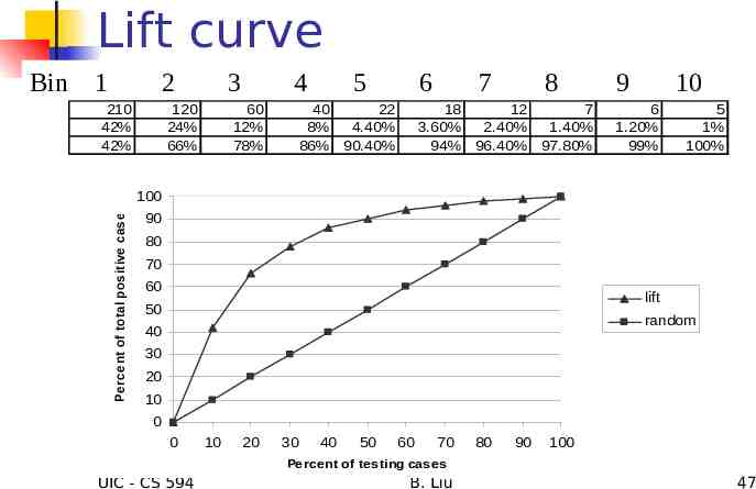
Lift curve 1 2 210 42% 42% 3 120 24% 66% 4 60 12% 78% 5 6 40 22 8% 4.40% 86% 90.40% 7 8 18 12 7 3.60% 2.40% 1.40% 94% 96.40% 97.80% 9 10 6 1.20% 99% 5 1% 100% 100 Pe rce nt of total pos itive cas e s Bin 90 80 70 60 lift 50 random 40 30 20 10 0 0 10 20 30 40 50 60 70 80 90 100 Percent of testing cases UIC - CS 594 B. Liu 47