CASSIE QUINN AND BRANDON BRUNNER 2017 MAYO DATA CHALLENGE 1


46 Slides2.13 MB
CASSIE QUINN AND BRANDON BRUNNER 2017 MAYO DATA CHALLENGE 1
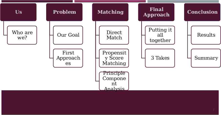
Us Who are we? Problem Matching Final Approach Conclusion Our Goal Direct Match Putting it all together Results First Approach es Propensit y Score Matching 3 Takes Summary Principle Compone nt Analysis 2
CASSIE QUINN Mathematics with Applied Emphasis Computer Science Minor Junior here at UW-La Crosse Expected to graduate Spring 2019! I enjoy the outdoors and dogs of all types. I am an avid Netflix-binger (specifically reality TV shows and The Office) and foodindulger. I ran a marathon last summer for a free t- shirt! Joined this project to gain a deeper perspective on the non-education Math world. 3
BRANDON BRUNNER Applied Physics Major Mathematics Minor Passion for analytical work involving machine learning and data analysis I enjoy spending quality time with my wife and Husky Senior at UW-La Crosse Expected to graduate in spring 2018 Joined Project to expand project portfolio and understanding of statistical methods 4
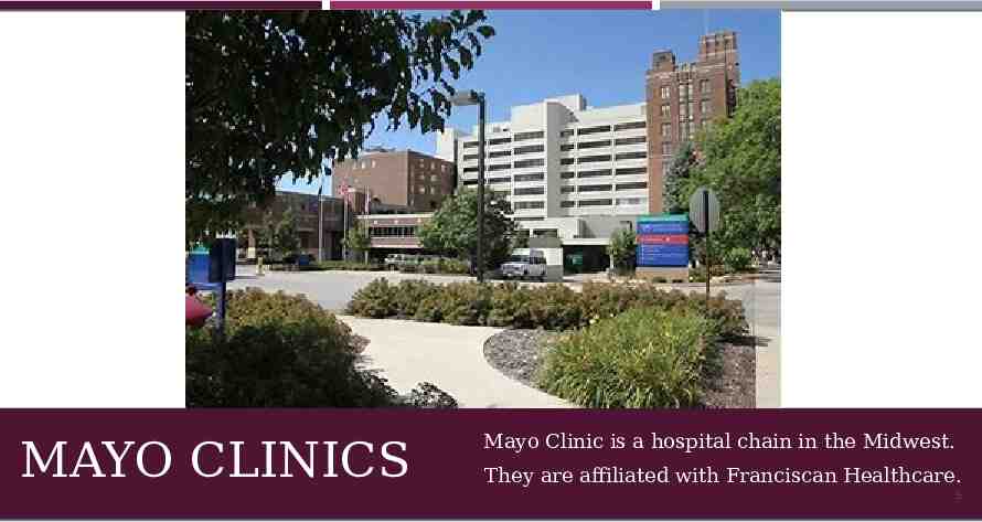
MAYO CLINICS Mayo Clinic is a hospital chain in the Midwest. They are affiliated with Franciscan Healthcare. 5
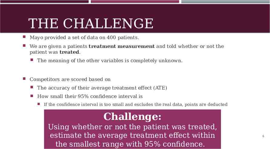
THE CHALLENGE Mayo provided a set of data on 400 patients. We are given a patients treatment measurement and told whether or not the patient was treated. The meaning of the other variables is completely unknown. Competitors are scored based on The accuracy of their average treatment effect (ATE) How small their 95% confidence interval is If the confidence interval is too small and excludes the real data, points are deducted Challenge: Using whether or not the patient was treated, estimate the average treatment effect within the smallest range with 95% confidence. 6
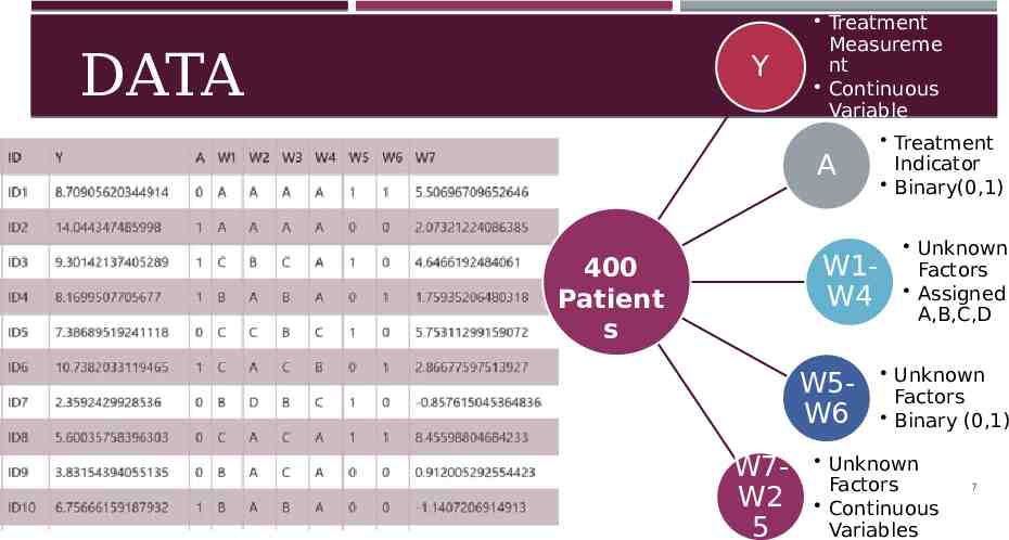
DATA Y Treatment Measureme nt Continuous Variable A W1W4 400 Patient s W5W6 W7W2 5 Treatment Indicator Binary(0,1) Unknown Factors Assigned A,B,C,D Unknown Factors Binary (0,1) Unknown Factors Continuous Variables 7
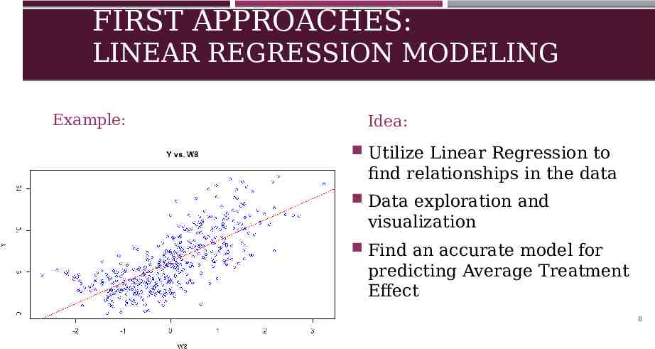
FIRST APPROACHES: LINEAR REGRESSION MODELING Example: EXAMPLE PIC OF ONE LINEAR REGRESSION MODEL Idea: Utilize Linear Regression to find relationships in the data Data exploration and visualization Find an accurate model for predicting Average Treatment Effect 8
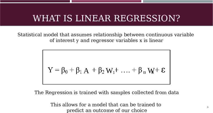
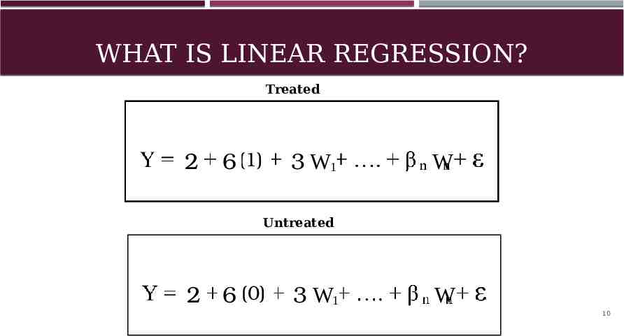
WHAT IS LINEAR REGRESSION? Statistical model that assumes relationship between continuous variable of interest y and regressor variables x is linear A W1 W The Regression is trained with samples collected from data This allows for a model that can be trained to predict an outcome of our choice 9
WHAT IS LINEAR REGRESSION? Treated 2 6 (1) A 3 W1 W Untreated 2 6 (0) A 3 W1 W 10
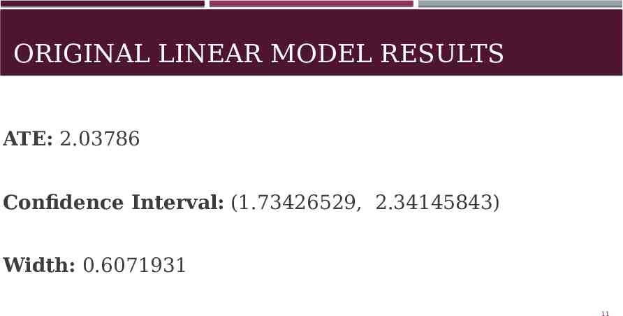
ORIGINAL LINEAR MODEL RESULTS ATE: 2.03786 Confidence Interval: (1.73426529, 2.34145843) Width: 0.6071931 11
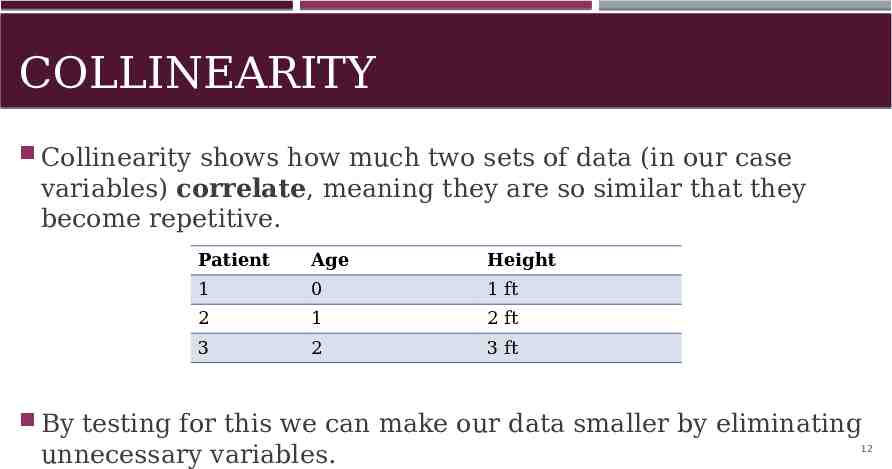
COLLINEARITY Collinearity shows how much two sets of data (in our case variables) correlate, meaning they are so similar that they become repetitive. Patient Age Height 1 0 1 ft 2 1 2 ft 3 2 3 ft By testing for this we can make our data smaller by eliminating unnecessary variables. 12
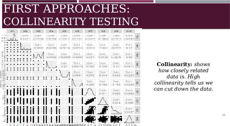
FIRST APPROACHES: COLLINEARITY TESTING Collinearity: shows how closely related data is. High collinearity tells us we can cut down the data. 13
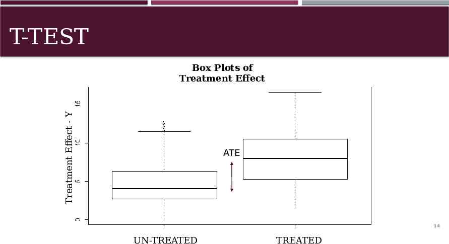
T-TEST Treatment Effect - Y Box Plots of Treatment Effect ATE 14 UN-TREATED TREATED
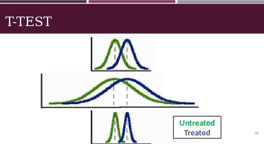
T-TEST Untreated Treated 15
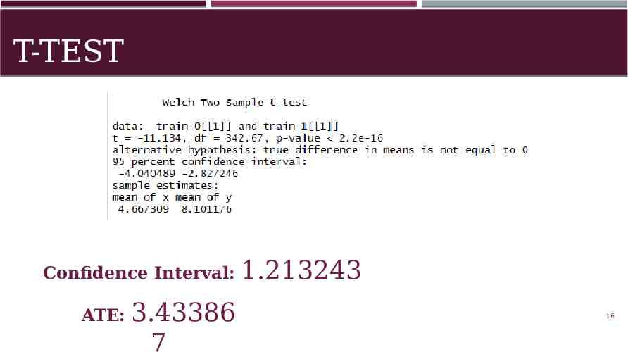
T-TEST Confidence Interval: ATE: 3.43386 7 1.213243 16
FIRST APPROACHES: OVERVIEW Playing with linear regression models with various aspects of the data to visualize relationships and get a better understanding of how the data worked together. Individual collinearity tests as well as overall collinearity testing to observe the variables closely related and potentially shrink size of our data. Using T-Tests to find the significance of the differences between treated and untreated groups. Overall, simply learning more about the data and observing patterns. 17
A FEW THINGS TO CONSIDER. Patient is either only treated or not Many unknown variables 18
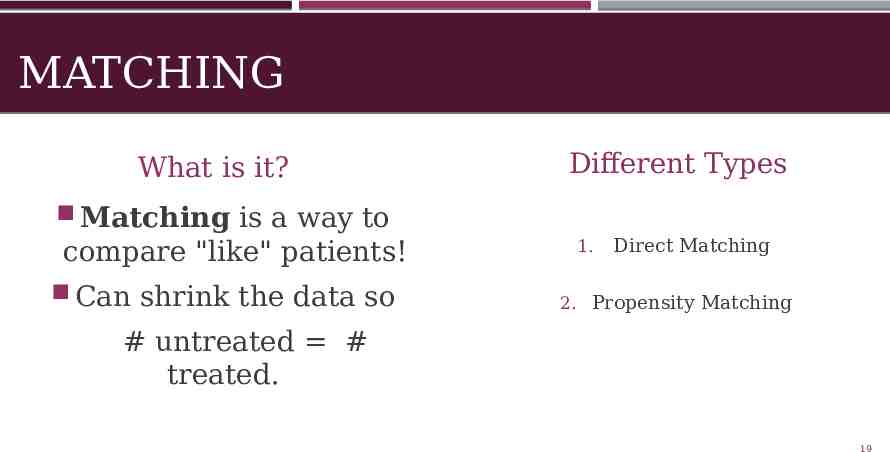
MATCHING What is it? Different Types Matching is a way to compare "like" patients! Can shrink the data so 1. Direct Matching 2. Propensity Matching # untreated # treated. 19
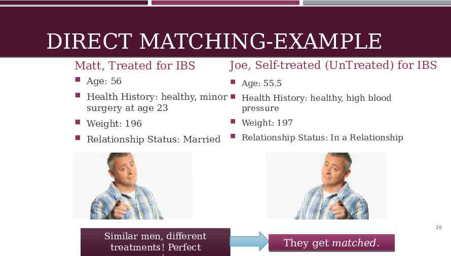
DIRECT MATCHING-EXAMPLE Matt, Treated for IBS Joe, Self-treated (UnTreated) for IBS Age: 56 Age: 55.5 Health History: healthy, minor Health History: healthy, high blood surgery at age 23 pressure Weight: 196 Weight: 197 Relationship Status: Married Relationship Status: In a Relationship 20 Similar men, different treatments! Perfect They get matched.
PROPENSITY MATCHING A patient can be only treated or not treated Is it logical to match two individuals directly based on unknown data? What if we could compare individuals based on their likelihood of treatment. 21
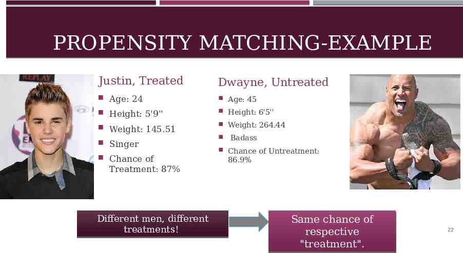
PROPENSITY MATCHING-EXAMPLE Justin, Treated Dwayne, Untreated Age: 24 Age: 45 Height: 5'9'' Height: 6'5'' Weight: 145.51 Weight: 264.44 Singer Chance of Badass Chance of Untreatment: 86.9% Treatment: 87% Different men, different treatments! Same chance of respective "treatment". 22
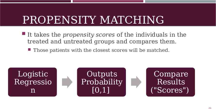
PROPENSITY MATCHING It takes the propensity scores of the individuals in the treated and untreated groups and compares them. Those patients with the closest scores will be matched. Logistic Regressio n Outputs Probability [0,1] Compare Results ("Scores") 23
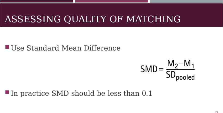
ASSESSING QUALITY OF MATCHING Use Standard Mean Difference In practice SMD should be less than 0.1 24
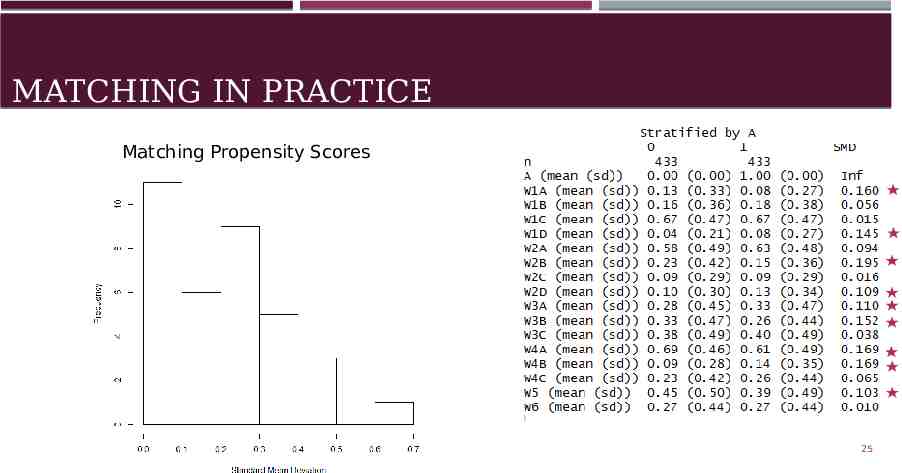
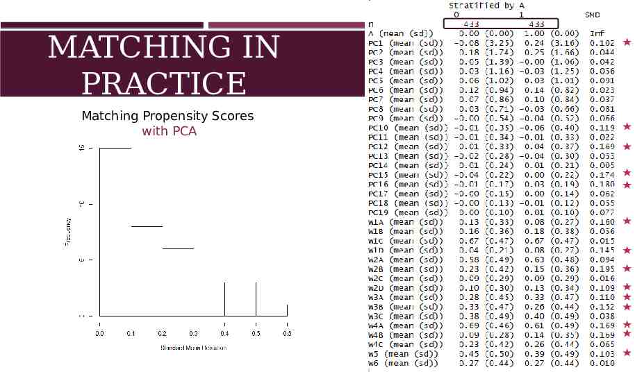
MATCHING IN PRACTICE Matching Propensity Scores Insert Table Without PCA (Just on Matched prop scores data) 25
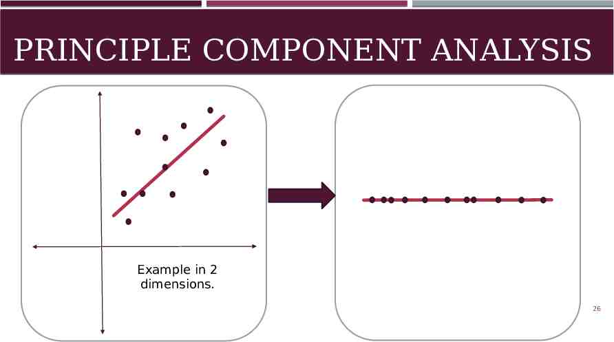
PRINCIPLE COMPONENT ANALYSIS Example in 2 dimensions. 26
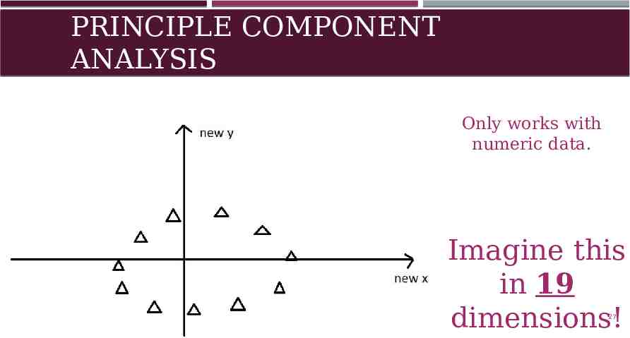
PRINCIPLE COMPONENT ANALYSIS Only works with numeric data. Imagine this in 19 dimensions! 27
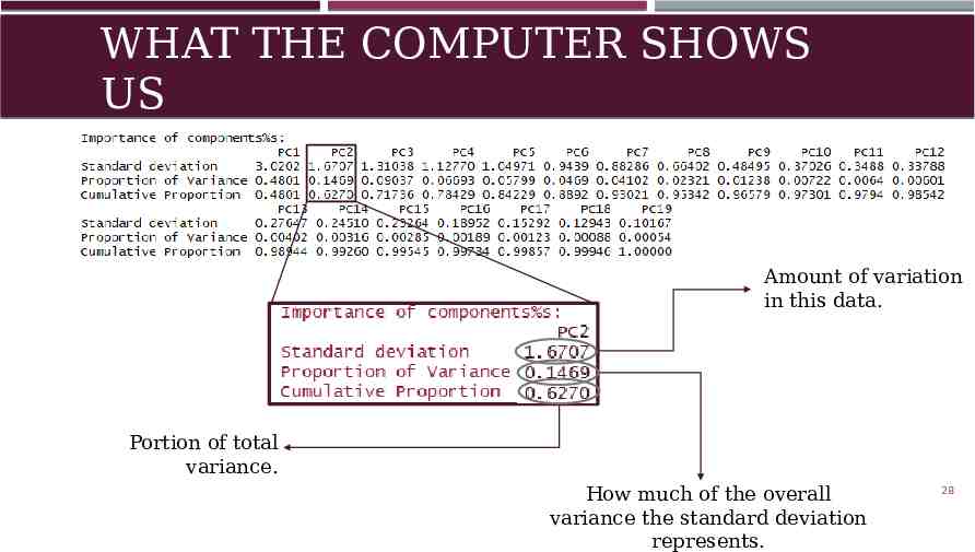
WHAT THE COMPUTER SHOWS US Amount of variation in this data. Portion of total variance. How much of the overall variance the standard deviation represents. 28
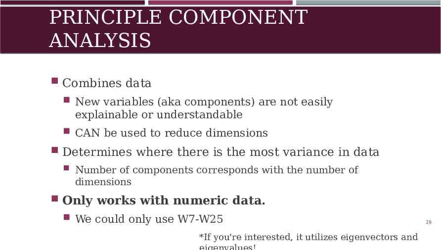
PRINCIPLE COMPONENT ANALYSIS Combines data New variables (aka components) are not easily explainable or understandable CAN be used to reduce dimensions Determines where there is the most variance in data Number of components corresponds with the number of dimensions Only works with numeric data. We could only use W7-W25 *If you're interested, it utilizes eigenvectors and 29
PUTTING IT ALL TOGETHER NOW. 30
MATCHING IN PRACTICE Matching Propensity Scores with PCA
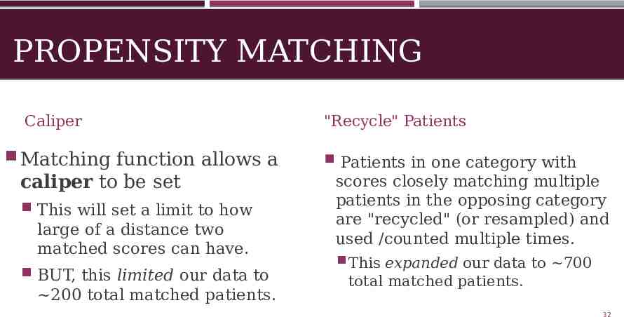
PROPENSITY MATCHING Caliper Matching function allows a caliper to be set This will set a limit to how large of a distance two matched scores can have. BUT, this limited our data to 200 total matched patients. "Recycle" Patients Patients in one category with scores closely matching multiple patients in the opposing category are "recycled" (or resampled) and used /counted multiple times. This expanded our data to 700 total matched patients. 32
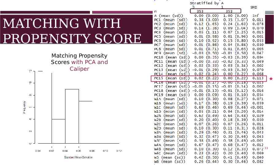
MATCHING WITH PROPENSITY SCORE Matching Propensity Scores with PCA and Caliper 33
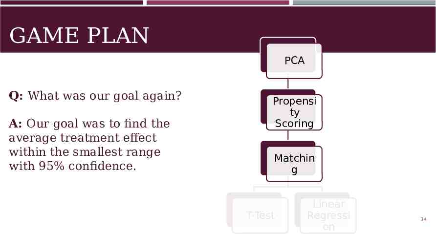
GAME PLAN PCA Q: What was our goal again? A: Our goal was to find the average treatment effect within the smallest range with 95% confidence. Propensi ty Scoring Matchin g T-Test Linear Regressi on 34
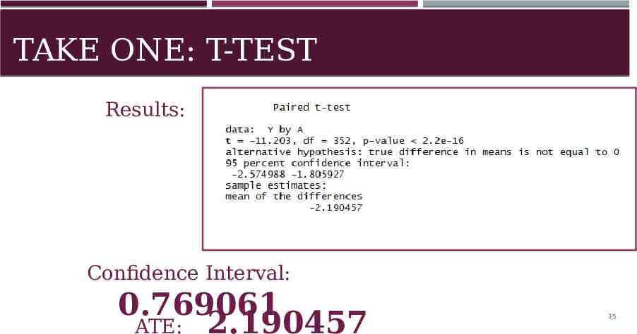
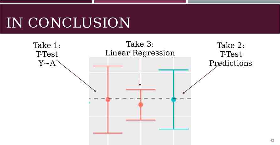
TAKE ONE: T-TEST Results: Confidence Interval: 0.769061 ATE: 2.190457 35
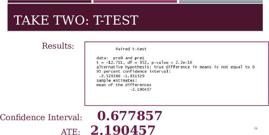
TAKE TWO: T-TEST Results: Confidence Interval: ATE: 0.677857 2.190457 36
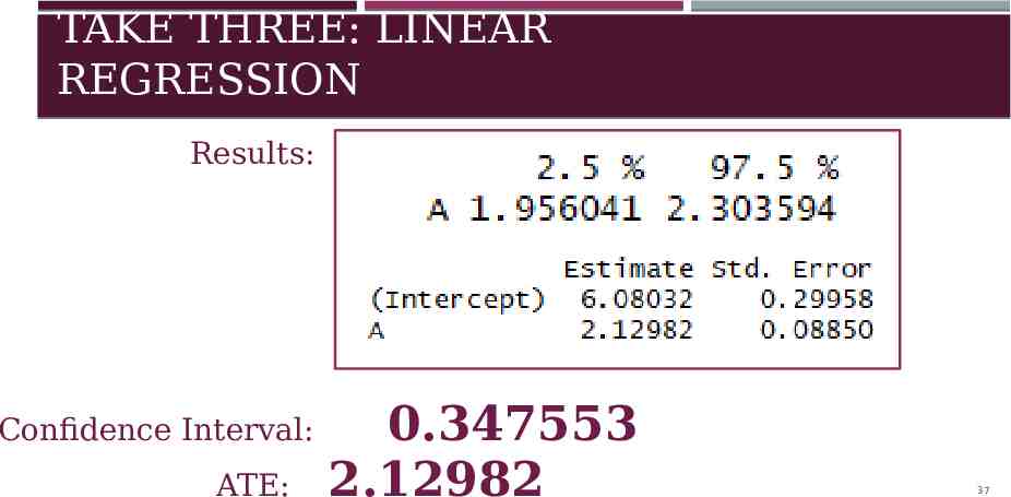
TAKE THREE: LINEAR REGRESSION Results: Confidence Interval: ATE: 0.347553 2.12982 37
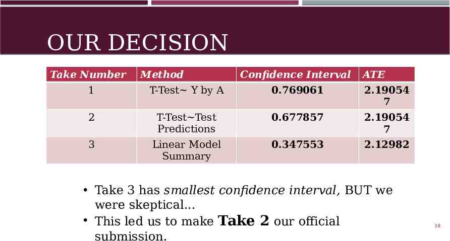
OUR DECISION Take Number Method Confidence Interval ATE 1 T-Test Y by A 0.769061 2.19054 7 2 T-Test Test Predictions 0.677857 2.19054 7 3 Linear Model Summary 0.347553 2.12982 Take 3 has smallest confidence interval, BUT we were skeptical. This led us to make Take 2 our official submission. 38
*DRUMROLL PLEASE* 39
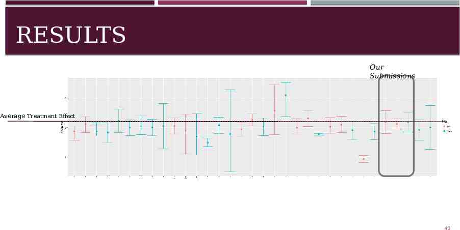
RESULTS Our Submissions Average Treatment Effect 40
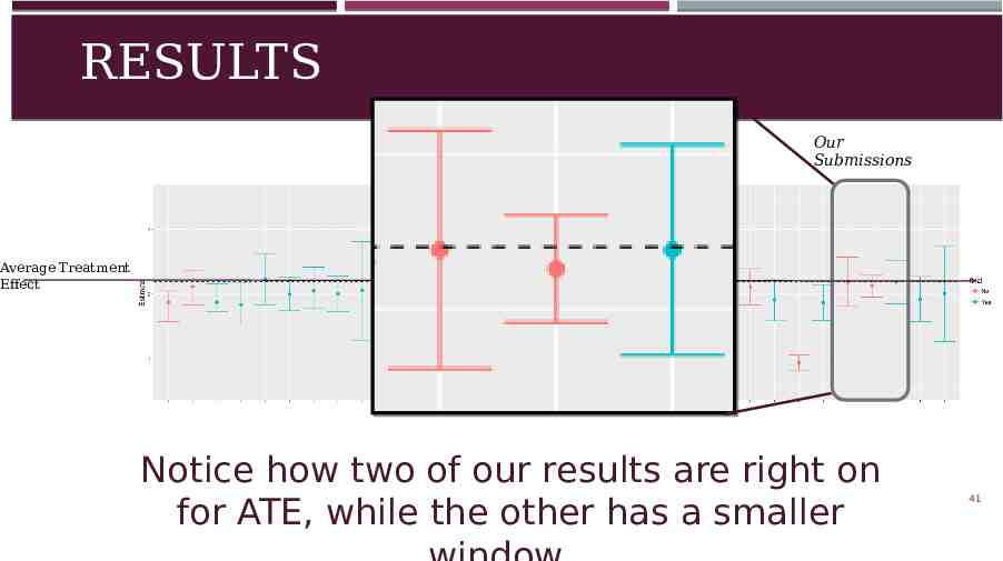
RESULTS Our Submissions Average Treatment Effect Notice how two of our results are right on for ATE, while the other has a smaller 41
IN CONCLUSION Take 1: T-Test Y A Take 3: Linear Regression Take 2: T-Test Predictions 42
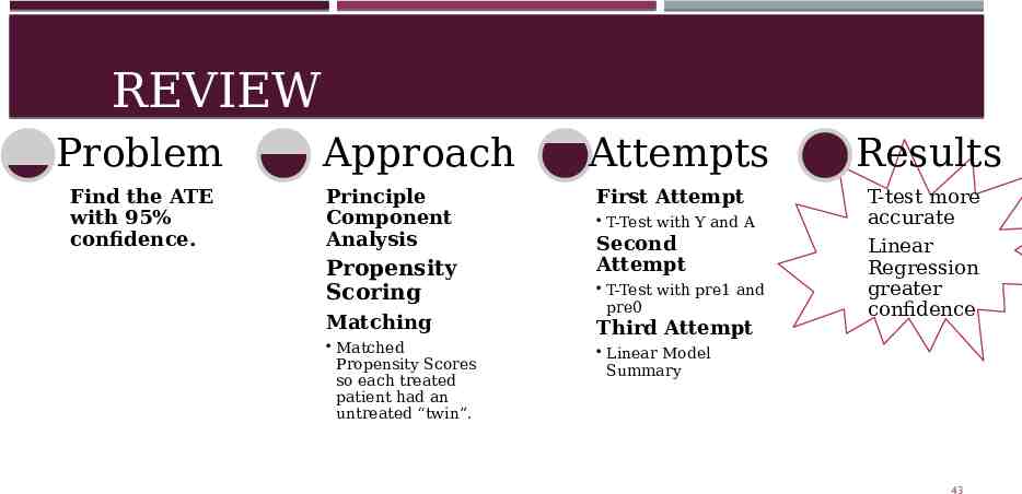
REVIEW Problem Find the ATE with 95% confidence. Approach Principle Component Analysis Propensity Scoring Matching Matched Propensity Scores so each treated patient had an untreated “twin”. Attempts First Attempt T-Test with Y and A Second Attempt T-Test with pre1 and pre0 Third Attempt Results T-test more accurate Linear Regression greater confidence Linear Model Summary 43
IN CONCLUSION We gained: Knowledge of new analyses Experience coding in R Working in a team Now: Still learning new analyses MTH 480-Applied Mathematics 44
ACKNOWLEDGEMENTS Dr. Chen and Dr. Vidden for their patience and guidance. A Crash Course in Causality: Inferring Causal Effects from Observational Data, University of Pennsylvania for its knowledge on Propensity Analysis T-test graph from Evan's Awesome A/B tools George Dallas for his wonderful graphs explaining PCA And of course.GOOGLE for its plethora of useful articles. 45
THANK YOU FOR COMING! -Cassie and Brandon