Supervised Learning Networks
43 Slides2.10 MB
Supervised Learning Networks
Supervised Learning Networks Linear perceptron networks Multi-layer perceptrons Mixture of experts Decision-based neural networks Hierarchical neural networks
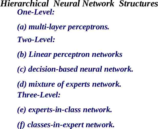
Hierarchical Neural Network Structures One-Level: (a) multi-layer perceptrons. Two-Level: (b) Linear perceptron networks (c) decision-based neural network. (d) mixture of experts network. Three-Level: (e) experts-in-class network. (f) classes-in-expert network.
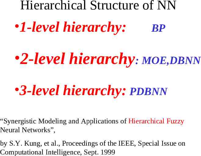
Hierarchical Structure of NN 1-level hierarchy: BP 2-level hierarchy: MOE,DBNN 3-level hierarchy: PDBNN “Synergistic Modeling and Applications of Hierarchical Fuzzy Neural Networks”, by S.Y. Kung, et al., Proceedings of the IEEE, Special Issue on Computational Intelligence, Sept. 1999
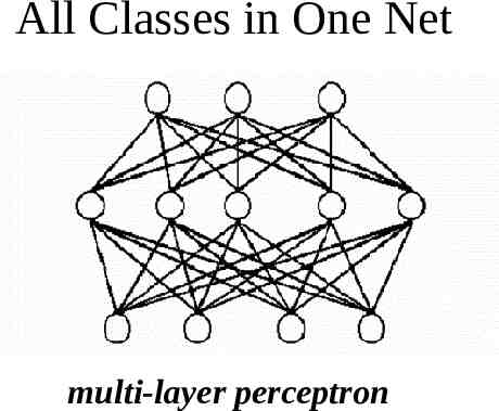
All Classes in One Net multi-layer perceptron
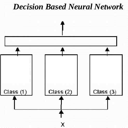
Modular Structures (two-level) Divide-and-conquer principle: divide the task into modules and then integrate the individual results into a collective decision. Two typical modular networks: (1) mixture-of-experts (MOE) which utilizes the expert-level modules, (2) decision-based neural networks (DBNN) based on the class-level modules.
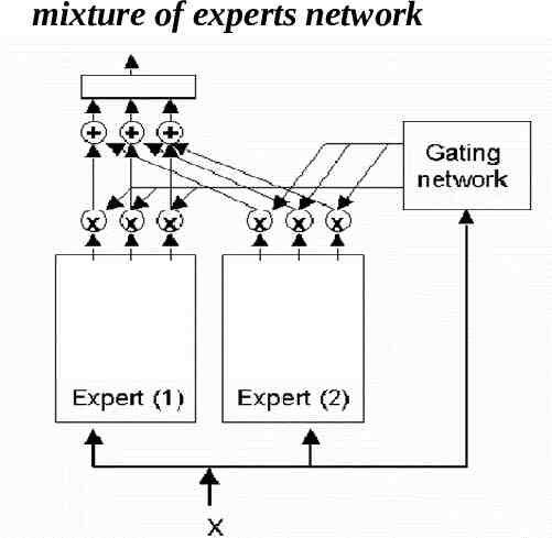
Expert-level (Rule-level) Modules: Each expert serves the function of (1) extracting local features and (2) making local recommendations. The rules in the gating network are used to decide how to combine recommendations from several local experts, with corresponding degree of confidences.
mixture of experts network
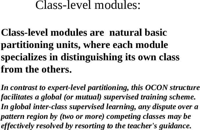
Class-level modules: Class-level modules are natural basic partitioning units, where each module specializes in distinguishing its own class from the others. In contrast to expert-level partitioning, this OCON structure facilitates a global (or mutual) supervised training scheme. In global inter-class supervised learning, any dispute over a pattern region by (two or more) competing classes may be effectively resolved by resorting to the teacher's guidance.
Decision Based Neural Network
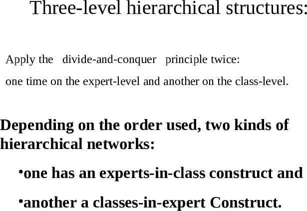
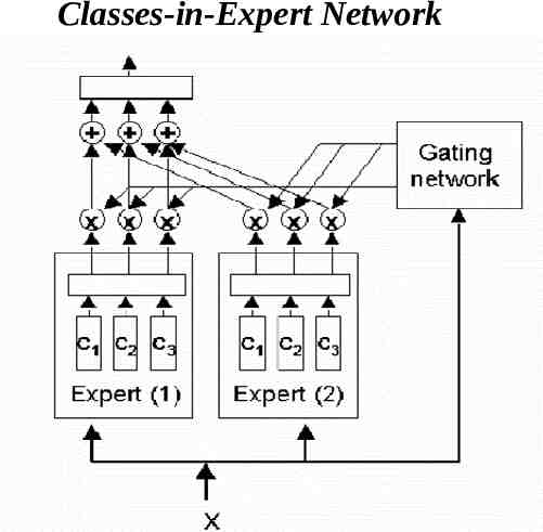
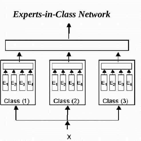
Three-level hierarchical structures: Apply the divide-and-conquer principle twice: one time on the expert-level and another on the class-level. Depending on the order used, two kinds of hierarchical networks: one has an experts-in-class construct and another a classes-in-expert Construct.
Classes-in-Expert Network
Experts-in-Class Network
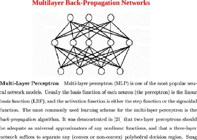
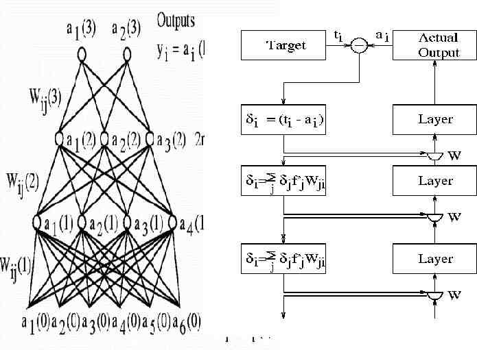
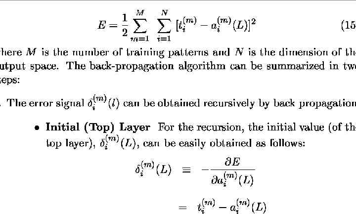
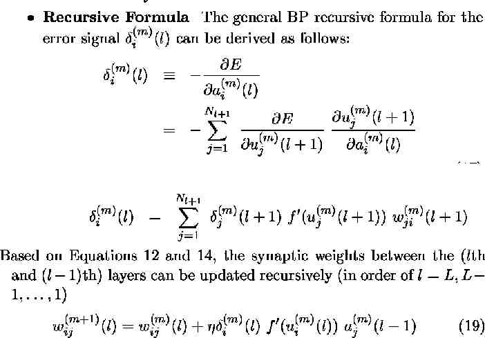
Multilayer Back-Propagation Networks
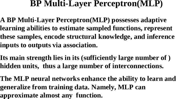
BP Multi-Layer Perceptron(MLP) A BP Multi-Layer Perceptron(MLP) possesses adaptive learning abilities to estimate sampled functions, represent these samples, encode structural knowledge, and inference inputs to outputs via association. Its main strength lies in its (sufficiently large number of ) hidden units, thus a large number of interconnections. The MLP neural networks enhance the ability to learn and generalize from training data. Namely, MLP can approximate almost any function.
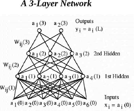
A 3-Layer Network
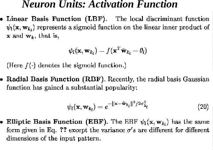
Neuron Units: Activation Function
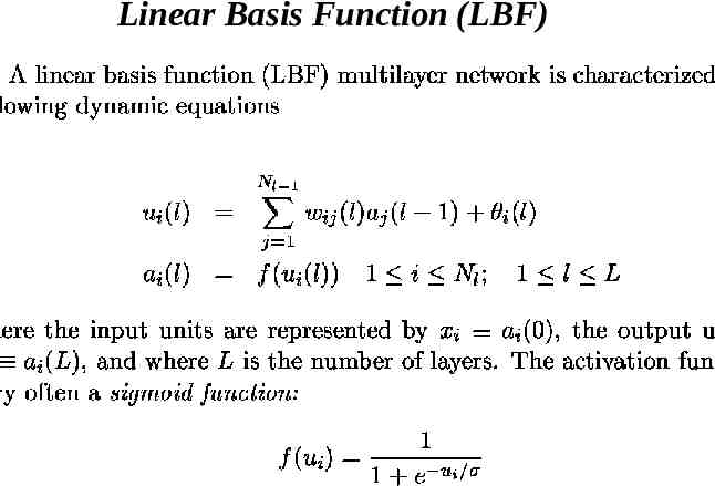
Linear Basis Function (LBF)
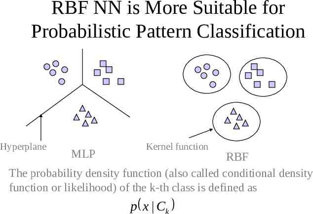
RBF NN is More Suitable for Probabilistic Pattern Classification Hyperplane MLP Kernel function RBF The probability density function (also called conditional density function or likelihood) of the k-th class is defined as p x Ck
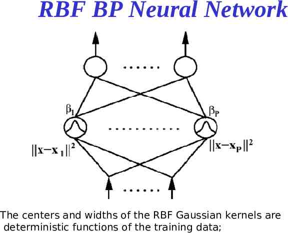
RBF BP Neural Network The centers and widths of the RBF Gaussian kernels are deterministic functions of the training data;
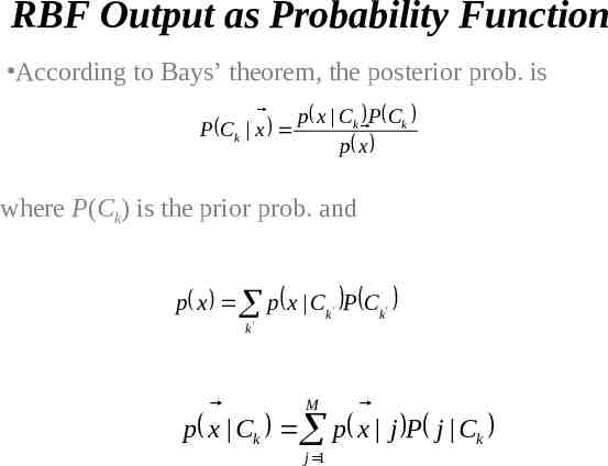
RBF Output as Probability Function According to Bays’ theorem, the posterior prob. is p x Ck P Ck P Ck x p x where P(Ck) is the prior prob. and p x p x Ck ' P Ck ' k' M p x Ck p x j P j Ck j 1
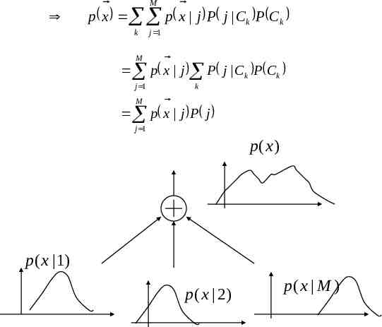
M p x p x j P j Ck P Ck k j 1 M p x j P j C k P C k j 1 k M p x j P j j 1 p(x ) p(x 1) p(x 2) p( x M )
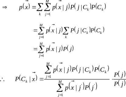
M p x p x j P j Ck P Ck k j 1 M p x j P j C k P C k j 1 k M p x j P j j 1 M p x j P j C k P Ck P Ck x j 1 M ' ' p x j P j j 1 P j P j
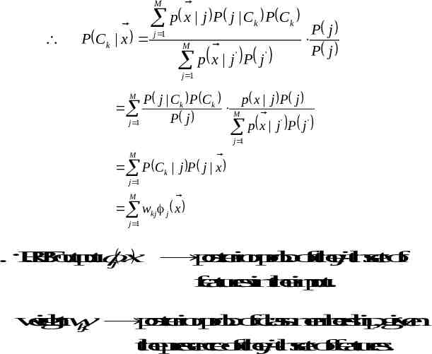
M p x j P j C k P Ck P Ck x j 1 M ' p x j P j' P j P j j 1 P j Ck P Ck p x j P j M ' P j ' j 1 p x j P j M j 1 M P C k j P j x j 1 M wkj j x j 1 R B F o u t p u t p o s t e r i o rp r o b .o ft h e j t h s e to f x j f e a t u r e s i n t h e i n p u t. w e i g h tw p o s t e r i o rp r o b .o fc l a s s m e m b e r s h i p ,g i v e n k j t h e p r e s e n c e o ft h e j t h s e to ff e a t u r e s .
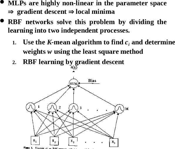
MLPs are highly non-linear in the parameter space gradient descent local minima RBF networks solve this problem by dividing the learning into two independent processes. 1. 2. Use the K-mean algorithm to find ci and determine weights w using the least square method RBF learning by gradient descent
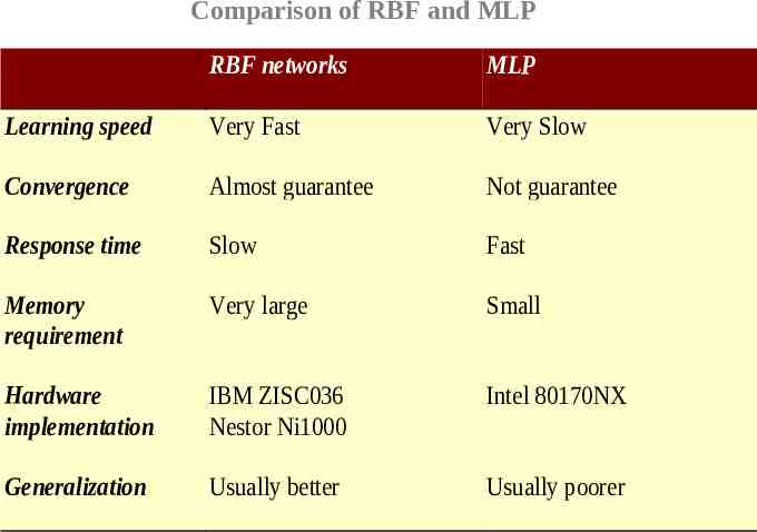
Comparison of RBF and MLP RBF networks MLP Learning speed Very Fast Very Slow Convergence Almost guarantee Not guarantee Response time Slow Fast Memory requirement Very large Small Hardware implementation IBM ZISC036 Nestor Ni1000 Intel 80170NX Generalization Usually better Usually poorer
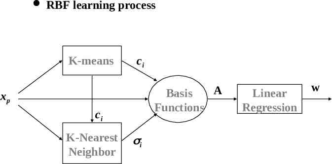
RBF learning process K-means ci A Basis Functions xp ci K-Nearest Neighbor i Linear Regression w
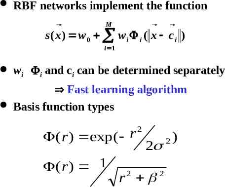
RBF networks implement the function M s( x ) w 0 w i i ( x c i ) i 1 wi i and ci can be determined separately Fast learning algorithm Basis function types 2 r ( r ) exp( ( r ) 1 2 r2 2 2 )
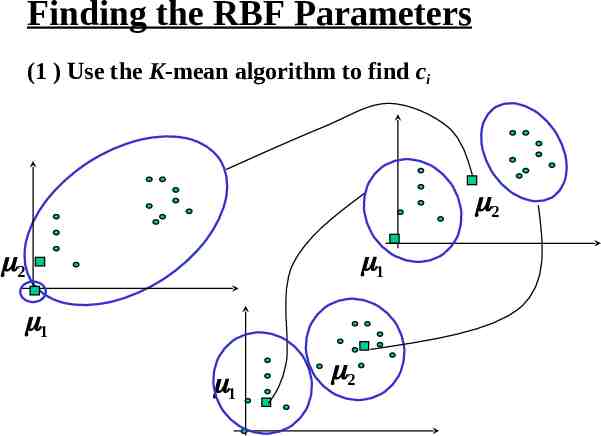
Finding the RBF Parameters (1 ) Use the K-mean algorithm to find ci 2 2 1 1 1 2
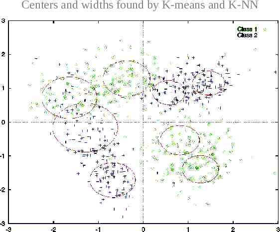
Centers and widths found by K-means and K-NN
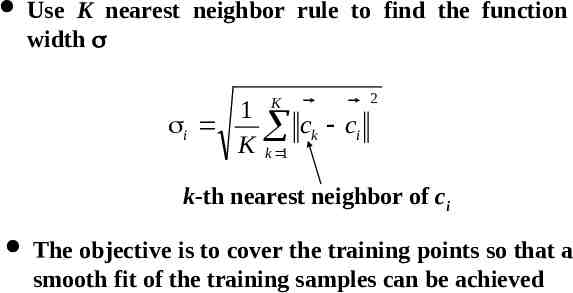
Use K nearest neighbor rule to find the function width 1 i K K ck ci 2 k 1 k-th nearest neighbor of ci The objective is to cover the training points so that a smooth fit of the training samples can be achieved
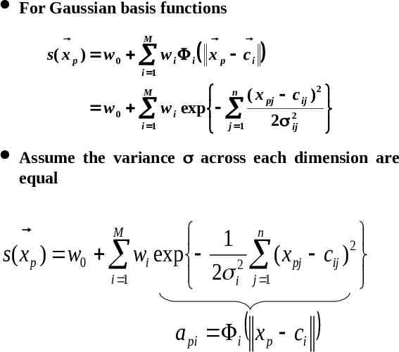
For Gaussian basis functions M s( x p ) w 0 w i i x p c i i 1 n ( x pj c ij ) 2 w 0 w i exp 2 2 ij i 1 j 1 M Assume the variance across each dimension are equal M 1 n 2 s ( x p ) w0 wi exp ( x pj cij ) 2 i 1 2 i j 1 a pi i x p ci
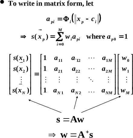
To write in matrix form, let a pi i x p c i M s( x p ) w i a pi where a p 0 1 i 0 s( x1 ) 1 a11 s( x ) 1 a 2 21 s( x ) 1 a N N1 a 12 a22 aN 2 a1 M w 0 a2 M w 1 a NM w M s Aw w A s
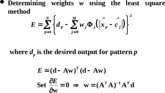
Determining weights w using the least square method 2 N M E d p w j j x p c j p 1 j 0 where dp is the desired output for pattern p E ( d Aw )T ( d Aw ) Set E 0 w ( A T A ) 1 A T d w
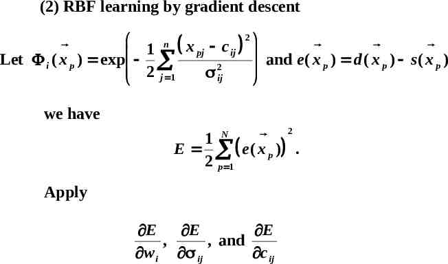
(2) RBF learning by gradient descent 2 n x pj c ij 1 and e ( x ) d ( x ) s( x ) Let i ( x p ) exp p p p 2 2 j 1 ij we have N 2 1 E e ( x p ) . 2 p 1 Apply E E E , , and w i ij c ij
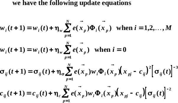
we have the following update equations N w i ( t 1) w i ( t ) w e ( x p ) i ( x p ) when i 1,2, , M p 1 N w i ( t 1) w i ( t ) w e ( x p ) when i 0 p 1 N 2 ij ( t 1) ij ( t ) e ( x p )w i i ( x p ) x pj c ij ij ( t ) p 1 N c ij ( t 1) c ij ( t ) c e ( x p )w i i ( x p ) x pj c ij ij ( t ) p 1 2 3
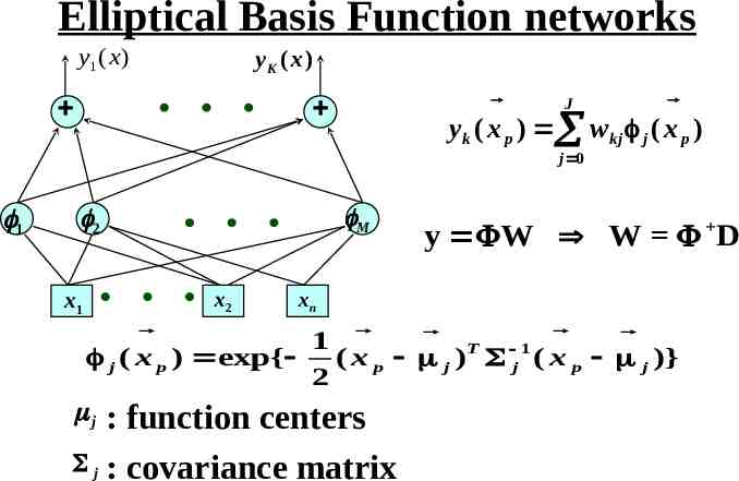
Elliptical Basis Function networks y1 ( x ) yK ( x ) J yk ( x p ) w kj j ( x p ) j 0 1 M 2 x1 x2 y W W D xn 1 j ( x p ) exp{ ( x p j )T j 1 ( x p j )} 2 : function centers j : covariance matrix j
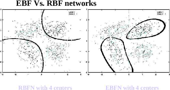
EBF Vs. RBF networks RBFN with 4 centers EBFN with 4 centers
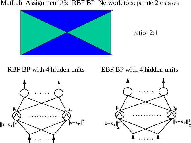
MatLab Assignment #3: RBF BP Network to separate 2 classes ratio 2:1 RBF BP with 4 hidden units EBF BP with 4 hidden units