Slides for Introduction to Stochastic Search and Optimization
29 Slides1.56 MB
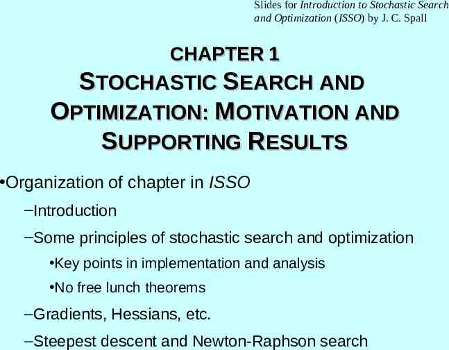
Slides for Introduction to Stochastic Search and Optimization (ISSO) by J. C. Spall CHAPTER 1 STOCHASTIC SEARCH AND OPTIMIZATION: MOTIVATION AND SUPPORTING RESULTS Organization of chapter in ISSO –Introduction –Some principles of stochastic search and optimization Key points in implementation and analysis No free lunch theorems –Gradients, Hessians, etc. –Steepest descent and Newton-Raphson search
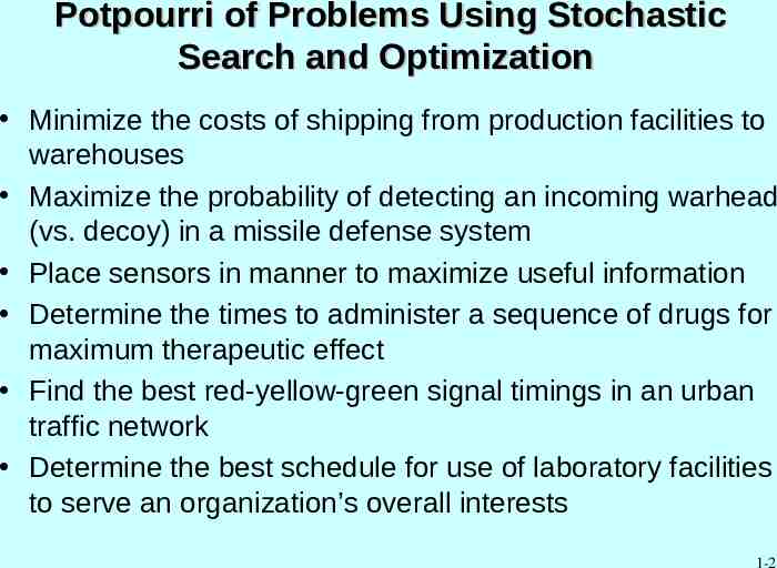
Potpourri of Problems Using Stochastic Search and Optimization Minimize the costs of shipping from production facilities to warehouses Maximize the probability of detecting an incoming warhead (vs. decoy) in a missile defense system Place sensors in manner to maximize useful information Determine the times to administer a sequence of drugs for maximum therapeutic effect Find the best red-yellow-green signal timings in an urban traffic network Determine the best schedule for use of laboratory facilities to serve an organization’s overall interests 1-2
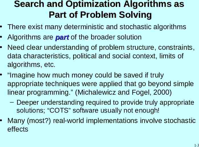
Search and Optimization Algorithms as Part of Problem Solving There exist many deterministic and stochastic algorithms Algorithms are part of the broader solution Need clear understanding of problem structure, constraints, data characteristics, political and social context, limits of algorithms, etc. “Imagine how much money could be saved if truly appropriate techniques were applied that go beyond simple linear programming.” (Michalewicz and Fogel, 2000) – Deeper understanding required to provide truly appropriate solutions; “COTS” software usually not enough! Many (most?) real-world implementations involve stochastic effects 1-3
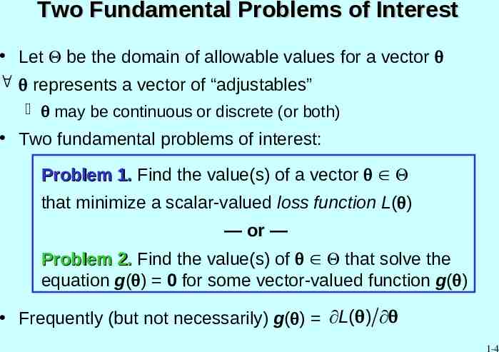
Two Fundamental Problems of Interest Let be the domain of allowable values for a vector represents a vector of “adjustables” may be continuous or discrete (or both) Two fundamental problems of interest: Problem 1. Find the value(s) of a vector that minimize a scalar-valued loss function L( ) — or — Problem 2. Find the value(s) of that solve the equation g( ) 0 for some vector-valued function g( ) Frequently (but not necessarily) g( ) L( ) 1-4
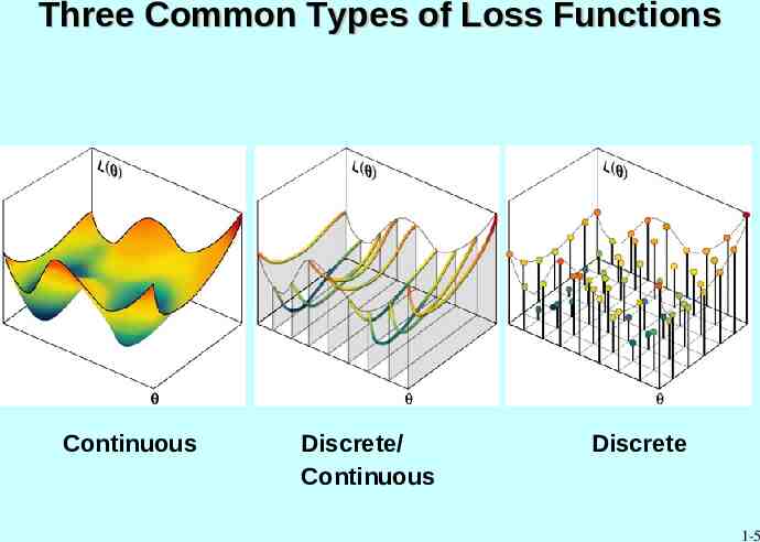
Three Common Types of Loss Functions Continuous Discrete/ Continuous Discrete 1-5
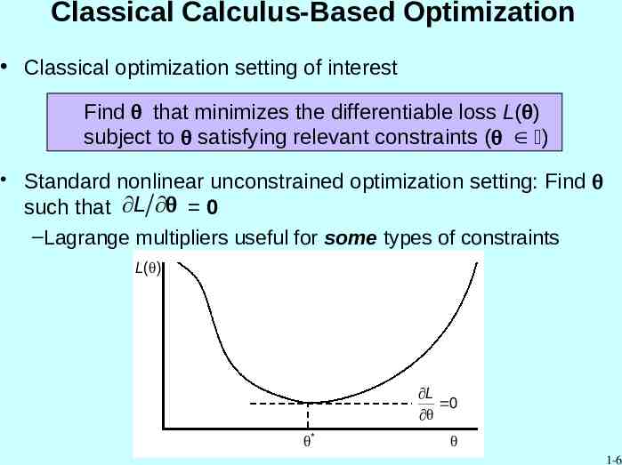
Classical Calculus-Based Optimization Classical optimization setting of interest Find that minimizes the differentiable loss L( ) subject to satisfying relevant constraints ( ) Standard nonlinear unconstrained optimization setting: Find such that L 0 –Lagrange multipliers useful for some types of constraints L( ) L 0 * 1-6
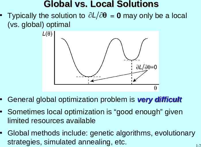
Global vs. Local Solutions Typically the solution to L 0 may only be a local (vs. global) optimal General global optimization problem is very difficult Sometimes local optimization is “good enough” given limited resources available Global methods include: genetic algorithms, evolutionary strategies, simulated annealing, etc. 1-7
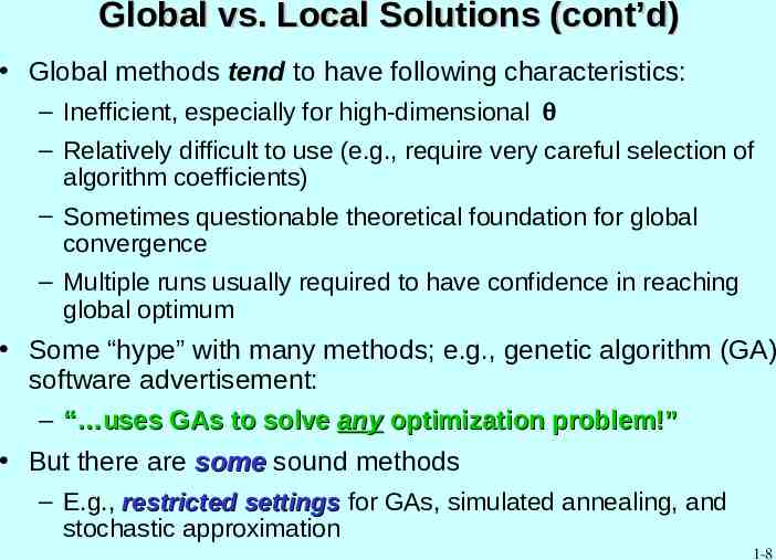
Global vs. Local Solutions (cont’d) Global methods tend to have following characteristics: – Inefficient, especially for high-dimensional – Relatively difficult to use (e.g., require very careful selection of algorithm coefficients) – Sometimes questionable theoretical foundation for global convergence – Multiple runs usually required to have confidence in reaching global optimum Some “hype” with many methods; e.g., genetic algorithm (GA) software advertisement: – “ uses GAs to solve any optimization problem!” But there are some sound methods – E.g., restricted settings for GAs, simulated annealing, and stochastic approximation 1-8
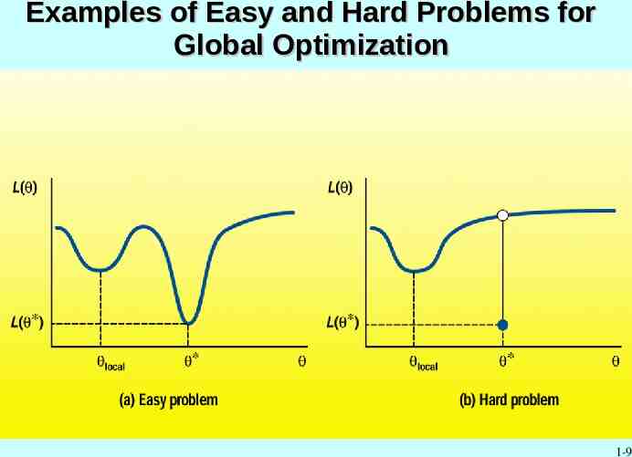
Examples of Easy and Hard Problems for Global Optimization 1-9
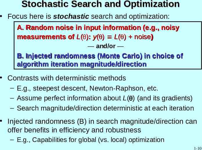
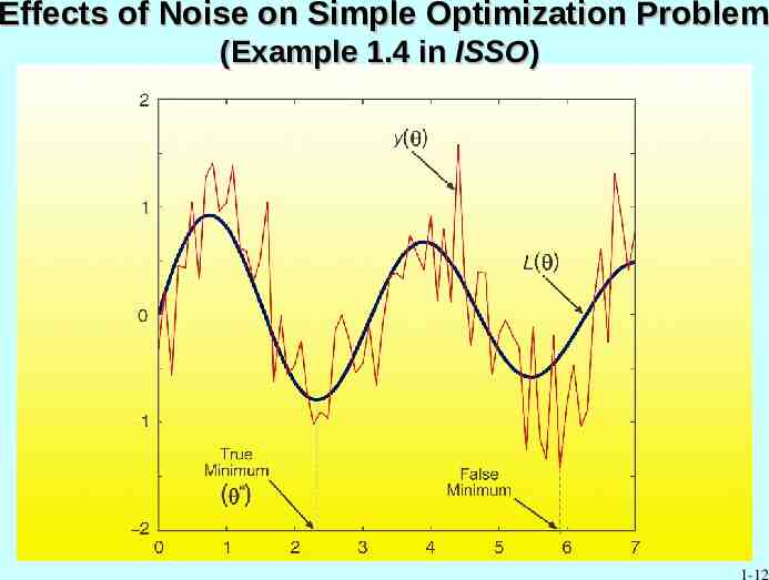
Stochastic Search and Optimization Focus here is stochastic search and optimization: A. Random noise in input information (e.g., noisy measurements of L( ): y( ) L( ) noise) — and/or — B. Injected randomness (Monte Carlo) in choice of algorithm iteration magnitude/direction Contrasts with deterministic methods – E.g., steepest descent, Newton-Raphson, etc. – Assume perfect information about L( ) (and its gradients) – Search magnitude/direction deterministic at each iteration Injected randomness (B) in search magnitude/direction can offer benefits in efficiency and robustness – E.g., Capabilities for global (vs. local) optimization 1-10
Some Popular Stochastic Search and Optimization Techniques Random search Stochastic approximation – – – – – – Robbins-Monro and Kiefer-Wolfowitz SPSA NN backpropagation Infinitesimal perturbation analysis Recursive least squares Many others Simulated annealing Genetic algorithms Evolutionary programs and strategies Reinforcement learning Markov chain Monte Carlo (MCMC) Etc. 1-11
Effects of Noise on Simple Optimization Problem (Example 1.4 in ISSO) 1-12
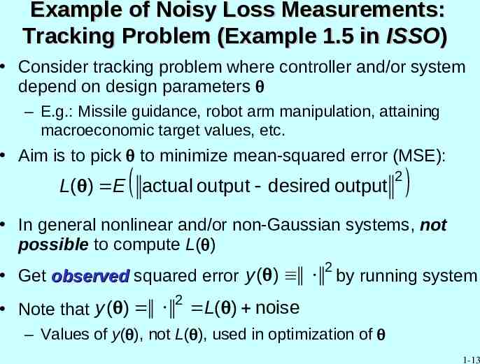
Example of Noisy Loss Measurements: Tracking Problem (Example 1.5 in ISSO) Consider tracking problem where controller and/or system depend on design parameters – E.g.: Missile guidance, robot arm manipulation, attaining macroeconomic target values, etc. Aim is to pick to minimize mean-squared error (MSE): L( ) E actual output desired output 2 In general nonlinear and/or non-Gaussian systems, not possible to compute L( ) Get observed squared error y ( ) Note that y ( ) 2 by running system 2 L( ) noise – Values of y( ), not L( ), used in optimization of 1-13
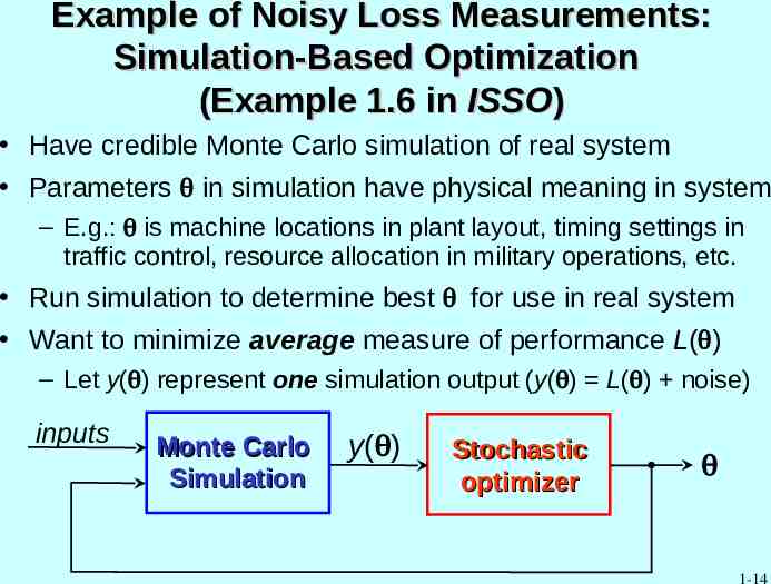
Example of Noisy Loss Measurements: Simulation-Based Optimization (Example 1.6 in ISSO) Have credible Monte Carlo simulation of real system Parameters in simulation have physical meaning in system – E.g.: is machine locations in plant layout, timing settings in traffic control, resource allocation in military operations, etc. Run simulation to determine best for use in real system Want to minimize average measure of performance L( ) – Let y( ) represent one simulation output (y( ) L( ) noise) inputs Monte Carlo Simulation y( ) Stochastic optimizer 1-14
Some Key Properties in Implementation and Evaluation of Stochastic Algorithms Algorithm comparisons via number of measurements of L( ) or g( ) (not iterations) – Function measurements typically represent major cost Curse of dimensionality – E.g.: If dim( ) 10, each element of can take on 10 values. Take 10,000 random samples: Prob(finding one of 500 best ) 0.0005 – Above example would be even much harder with only noisy function measurements Constraints Limits of numerical comparisons – Avoid broad claims based on numerical studies – Best to combine theory and numerical analysis 1-15
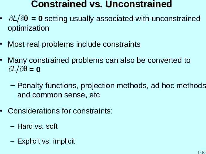
Constrained vs. Unconstrained L 0 setting usually associated with unconstrained optimization Most real problems include constraints Many constrained problems can also be converted to L 0 – Penalty functions, projection methods, ad hoc methods and common sense, etc Considerations for constraints: – Hard vs. soft – Explicit vs. implicit 1-16
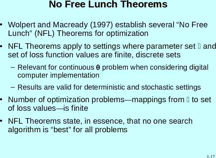
No Free Lunch Theorems Wolpert and Macready (1997) establish several “No Free Lunch” (NFL) Theorems for optimization NFL Theorems apply to settings where parameter set and set of loss function values are finite, discrete sets – Relevant for continuous problem when considering digital computer implementation – Results are valid for deterministic and stochastic settings Number of optimization problems—mappings from to set of loss values—is finite NFL Theorems state, in essence, that no one search algorithm is “best” for all problems 1-17
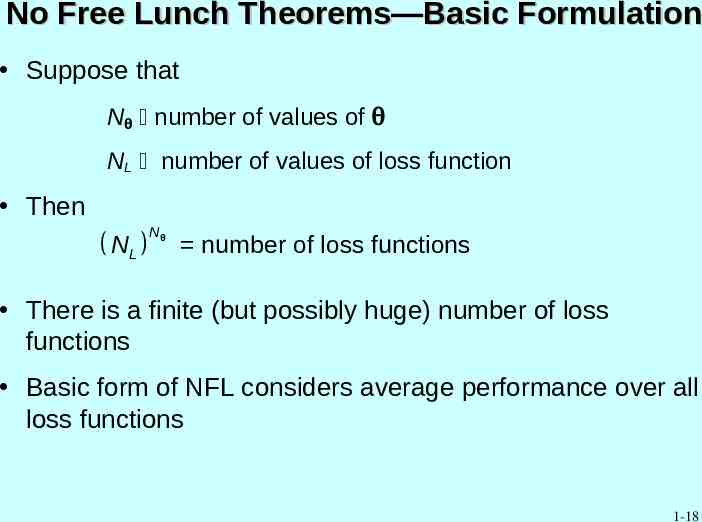
No Free Lunch Theorems—Basic Formulation Suppose that N number of values of NL number of values of loss function Then NL Nθ number of loss functions There is a finite (but possibly huge) number of loss functions Basic form of NFL considers average performance over all loss functions 1-18
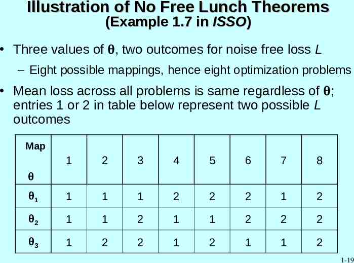
Illustration of No Free Lunch Theorems (Example 1.7 in ISSO) Three values of , two outcomes for noise free loss L – Eight possible mappings, hence eight optimization problems Mean loss across all problems is same regardless of ; entries 1 or 2 in table below represent two possible L outcomes Map 1 2 3 4 5 6 7 8 1 1 1 1 2 2 2 1 2 2 1 1 2 1 1 2 2 2 3 1 2 2 1 2 1 1 2 1-19
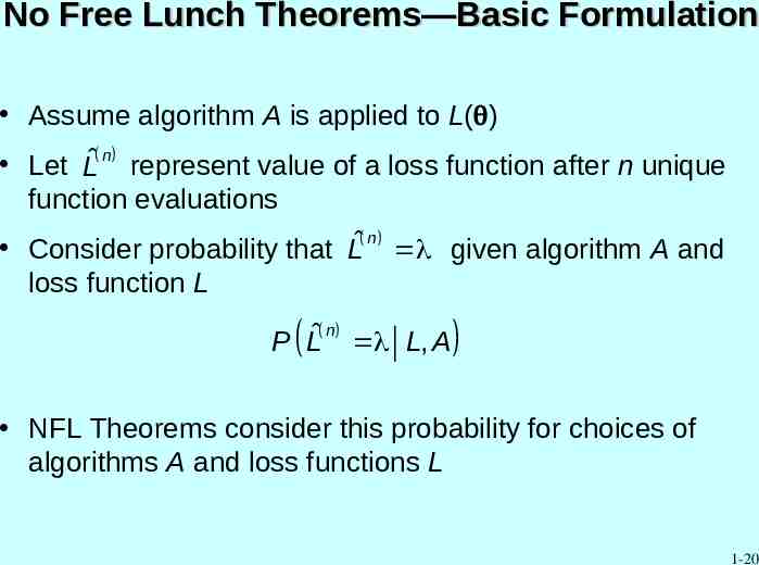
No Free Lunch Theorems—Basic Formulation Assume algorithm A is applied to L( ) Let Lˆ n represent value of a loss function after n unique function evaluations Consider probability that Lˆ n given algorithm A and loss function L n ˆ P L L, A NFL Theorems consider this probability for choices of algorithms A and loss functions L 1-20
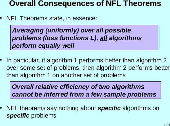
Overall Consequences of NFL Theorems NFL Theorems state, in essence: Averaging (uniformly) over all possible problems (loss functions L), all algorithms perform equally well In particular, if algorithm 1 performs better than algorithm 2 over some set of problems, then algorithm 2 performs better than algorithm 1 on another set of problems Overall relative efficiency of two algorithms cannot be inferred from a few sample problems NFL theorems say nothing about specific algorithms on specific problems 1-21
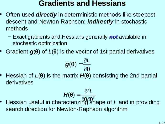
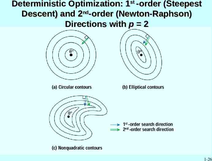
Gradients and Hessians Often used directly in deterministic methods like steepest descent and Newton-Raphson; indirectly in stochastic methods – Exact gradients and Hessians generally not available in stochastic optimization Gradient g( ) of L( ) is the vector of 1st partial derivatives L g ( ) Hessian of L( ) is the matrix H( ) consisting the 2nd partial derivatives 2L H ( ) T Hessian useful in characterizing shape of L and in providing search direction for Newton-Raphson algorithm 1-22
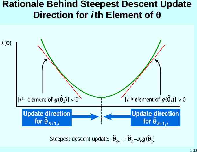
Rationale Behind Steepest Descent Update Direction for i th Element of 1-23
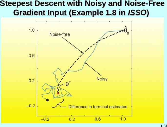
Steepest Descent with Noisy and Noise-Free Gradient Input (Example 1.8 in ISSO) 1-24
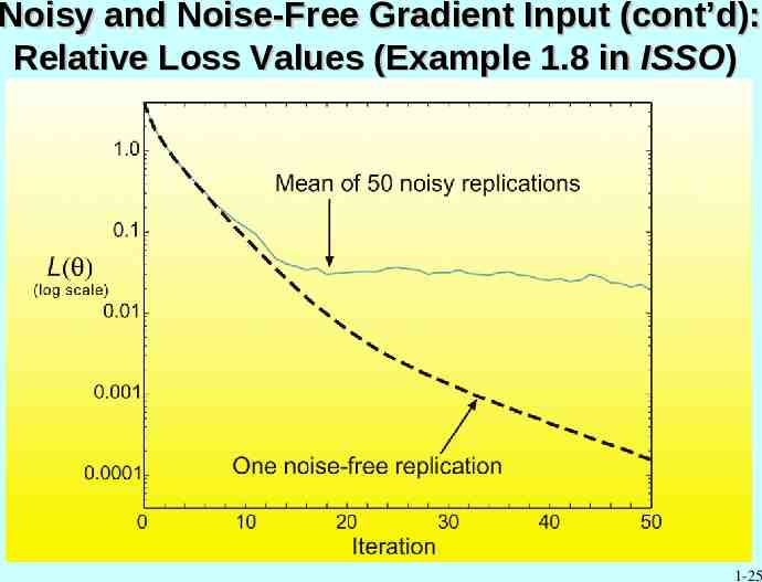
Noisy and Noise-Free Gradient Input (cont’d): Relative Loss Values (Example 1.8 in ISSO) 1-25
Deterministic Optimization: 1st -order (Steepest Descent) and 2nd-order (Newton-Raphson) Directions with p 2 1-26
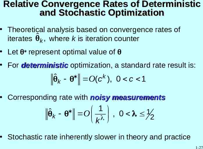
Relative Convergence Rates of Deterministic and Stochastic Optimization Theoretical analysis based on convergence rates of iterates ˆ k , where k is iteration counter Let represent optimal value of For deterministic optimization, a standard rate result is: ˆ k O(c k ), 0 c 1 Corresponding rate with noisy measurements ˆ k O 1 , 0 1 2 k Stochastic rate inherently slower in theory and practice 1-27
Concluding Remarks Stochastic search and optimization very widely used – Handles noise in the function evaluations – Generally better for global optimization – Broader applicability to “non-nice” problems (robustness) Some challenges in practical problems – – – – Noise dramatically affects convergence Distinguishing global from local minima not generally easy Curse of dimensionality Choosing algorithm “tuning coefficients” Rarely sufficient to use theory for standard deterministic methods to characterize stochastic methods “No free lunch” theorems are barrier to exaggerated claims of power and efficiency of any specific algorithm Algorithms should be implemented in context: “Better a rough answer to the right question than an exact answer to the wrong one” (Lord Kelvin) 1-28
Selected References on Stochastic Optimization Fogel, D. B. (2000), Evolutionary Computation: Toward a New Philosophy of Machine Intelligence (2nd ed.), IEEE Press, Piscataway, NJ. Fu, M. C. (2002), “Optimization for Simulation: Theory vs. Practice” (with discussion by S. Andradóttir, P. Glynn, and J. P. Kelly), INFORMS Journal on Computing, vol. 14, pp. 192 227. Goldberg, D. E. (1989), Genetic Algorithms in Search, Optimization, and Machine Learning, Addison-Wesley, Reading, MA. Gosavi, A. (2003), Simulation-Based Optimization: Parametric Optimization Techniques and Reinforcement Learning, Kluwer, Boston. Holland, J. H. (1975), Adaptation in Natural and Artificial Systems, University of Michigan Press, Ann Arbor, MI. Kushner, H. J. and Yin, G. G. (2003), Stochastic Approximation and Recursive Algorithms and Applications (2nd ed.), Springer-Verlag, New York. Michalewicz, Z. and Fogel, D. B. (2000), How to Solve It: Modern Heuristics, Springer-Verlag, New York. Spall, J. C. (2003), Introduction to Stochastic Search and Optimization: Estimation, Simulation, and Control, Wiley, Hoboken, NJ. Zhigljavsky, A. A. (1991), Theory of Global Random Search, Kluwer Academic, Boston. 1-29