NANO-MECHANICS BASED ASSESSMENT OF FAILURE RISK, SIZE EFFECT


41 Slides2.59 MB
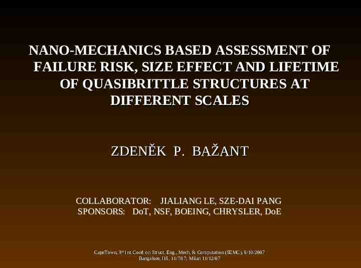
NANO-MECHANICS BASED ASSESSMENT OF FAILURE RISK, SIZE EFFECT AND LIFETIME OF QUASIBRITTLE STRUCTURES AT DIFFERENT SCALES ZDENĚK P. BAŽANT COLLABORATOR: JIALIANG LE, SZE-DAI PANG SPONSORS: DoT, NSF, BOEING, CHRYSLER, DoE CapeTown, CapeTown, 33rdrd Int. Int. Conf. Conf. on on Struct. Struct. Eng., Eng., Mech, Mech, & & Computation Computation (SEMC), (SEMC), 9/10/2007 9/10/2007 Bangalore, IIS, 11/7/07; Milan 11/12/07 Bangalore, IIS, 11/7/07; Milan 11/12/07
Energetic ( Quasibrittle ) Mean Size Effect Laws and Statistical Generalization 1c, 2c, 3c – based on cohesive crack model, 1 Type 2 1 r N 1 r 1 rk , 0 2 0.1 0.1 1 Type 1 1 1 N D 1 0 D0 1 2 Type 3 FM LE log ( Nom. Strength N ) 2c 3c N D1 D 0 D1 D D0 1s – statistical generalization Db Db D 1s m 1c 0.1 1 2 1r N n m rk 0 Weibul n l Statistical 10 100 log (Size D) 1 10 100
Failure at Crack Initiation: Type 1 EnergeticStatistical Size Effect on Strength and Lifetime
Importance of Tail Distribution of Pf Prob. of Failure 1 Same mean, same Gaussian cdf Tolerable failure prob. Pf 10-6 Pf 1 – exp[-(σ/ m] Weibull Mean cdf σ/ 1 0 TW TG Load
Definition: A structure is quasibrittle if Weibull cdf applies for sizes 104 equivalent RVEs Hypotheses: I. Interatomic bond energies have Maxwell-Boltzmann distribution, and activation energy depends on stress. II. Tests of lab specimens 5 RVEs do not disagree with Gaussian pdf.
Flaw Size Distribution: —physical justification of Weibull statistics? NO Why? Merely relates macro-level to micro-level hypotheses: 1. Noninteracting flaws, one in one volume element 2. Griffith (not cohesive!) theory holds on micro-level. ( a / u ) p 3. Cauchy distribution of flaw sizes: e Both fatigued polycrystalline metal and concrete are brittle, follow Weibull pdf, yet the flaws cannot be identified concrete.
1) pdf of One RVE
Atomistic Basis of cdf of Quasibrittle RVE Q / kT Maxwell-Boltzmann distribution f e frequency of exceeding activation energy Q ( Q ) / kT ( Q ) / kT e e 1) Net rate of breaks Interatomic pot. E 1 0 Q -assumed linear x breaks restorations Q / kT 2e sinh kT 2) Critical fraction of broken bonds b reached within stress duration 3) cdf of break surface: Pf 1 i Fs min Cb sinh , 1 kT Fs Tail Cb kT Q kT Cb 2 b e 0
plastic softening brittle (reality) long chains Power Law Tail of cdf of Strength b) Parallel Coupling 1 2 a) Series Coupling N (c) 12 n If each link has tail m, the p If each fiber has tail , chain has the the bundle has tail np same tail m additive exponents The reach of power-law tail is decreased drastically by parallel coupling, increased by series coupling. Parallel coupling produces cdf with Gaussian core. Power-law tail with zero threshold is indestructible!
Power Tail Length for Bundles & Chains 1) Brittle bundle with n 24 fibers (Daniels' model, 1945) having Weibull cdf with p 1 Gaussian core down to 0.3 Power tail up to 10-45 irrelevant! (D (l.y.)3) 2) Plastic bundle with n 24 fibers (Central Limit Theorem) having Weibull cdf with p 1 Gaussian core down to 0.01 Power tail up to 10-45 irrelevant! 3) Brittle bundle with n 2 fibers having Weibull cdf with p 12 Gaussian core down to 0.3 Power tail up to 5x10⁻⁵ longer but not enough 4) Plastic bundle with n 2 fibers having Weibull cdf with p 12 Gaussian core down to 0.3 Power tail up to 3x10⁻³ Plastic fibers extend Weibull tail to 3x10⁻³ . OK! Hence, a hierarchy of parallel series couplings is required!
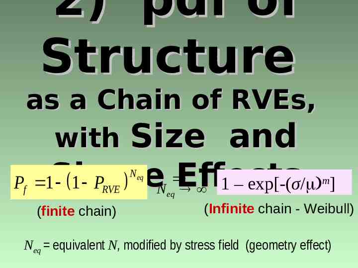
2) pdf of Structure as a Chain of RVEs, with Size and ShapeN Effects 1 – exp[-(σ/ ] Pf 1 1 PRVE (finite chain) N eq m eq (Infinite chain - Weibull) Neq equivalent N, modified by stress field (geometry effect)
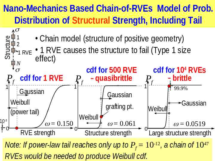
Nano-Mechanics Based Chain-of-RVEs Model of Prob. Distribution of Structural Strength, Including Tail Structure 1 2 1 RVE N Chain model (structure of positive geometry) 1 RVE causes the structure to fail (Type 1 size effect) Pf cdf for 1 RVE 1 Gaussian cdf for 500 RVE Pf quasibrittle 1 Weibull (power tail) 10-3 0 0.150 0 RVE strength cdf for 104 RVEs brittle Pf 1 99.9% Gaussian grafting pt. Weibull 0.061 Structure strength Weibull Gaussian 0.0519 0 Large structure strength Note: If power-law tail reaches only up to Pf 10-12, a chain of 1047 RVEs would be needed to produce Weibull cdf.
Quasi-Brittleness or Threshold Strength? Optimum fit by Weibull cdf Optimum fit by chain–of– with finite threshold RVEs, zero threshold ndata (2 days) 680 ndata (7 days) 1082 ndata (14 days) 1106 2 Pf 0.65 KINK - classical Weibull theory can’t explain -2 ln[- ln(1- Pf )] 1 3.6 7d ay s 28 da y 4.6 s A 2 d ge ay s 1 1 1.5 0.5 -6 5.3 1 1 Despite using threshold to optimize fit, Weibull theory can only fit tail m 16 m 24 m 20 1 -6 2.5 -2 (s - s ) ln(ln u)u Weibull cdf with N u finite threshold: Pf 1 e S0 3.5 Weibull scale ln[ ln(1 Pf)] 2 Weibull (1939) tests of Portland cement mortar 2.4 2.8 3.2 m RVE size 0.6 1.0 cm Specimen vol. 100 3000 cm3 ln(s ) ln 3.6 Pgr 0.0001 0.01 4.0
cdf of Structure Strength in Weibull Scale Pf 1 1 PRVE (finite chain) 1 RVE N Now: Fit by chain–of– RVEs, zero threshold Pf 0.65 1.5 7d 1 ln[- ln(1- Pf )] 5.3 2.5 A 2 d ge ay ay s s 28 da ys 1 4.6 3 ln( u) 2.4 2.8 3.2 102 -2 -4 m 24 1 -6 Gaussian 101 Neq 1 0 KINK - classical Weibull theory -2 1 can’t explain 1 16 20 3.6 -2 10 10 5 2 1 0.5 (Infinite chain - Weibull) 2 3.5 ln[ ln(1 Pf)] Weibull (1939) tests of Portland cement mortar -6 N eq 1 – exp[-(σ/ m] Neq equivalent N, modified by stress field (geometry effect) Previously: Fit by Weibull cdf with finite threshold 2 N eq lnln(s ) 3.6 -6 Weib ull Structure 1 2 Increasing size -8 4.0 -1.0 -0.6 Kink used to determine size of RVE and Pgr -0.2 ln(s N /S 0 ) ln( / S0) 0.2
Consequences of Chain-of-RVEs Model for Structural Strength 1) Threshold of power-law tail must be 0, i.e. Pf ( u ) n u 0 ! 105 103 2) 3) 2 Mean size 0.4 Failure Prob. 10 cdf of strength have kinks at the grafting points, moving up with size (# of RVEs) Neq 1 -2 -4 -6 Pgr 0.001 0.003 0.005 0.010 0.2 effect deviation from power law sets Pgr 0.0 log (size) Strength 5) Calculate safety factor for Pf 10-6 as a function of equiv. # of RVEs 0 0.3 C.o.V. of strength can increase or decrease decreases with 0 0.2 structural size 0 0.1 (# of RVEs) -8 -1.0 4) 1 0 10 0 log(m /S ) log(strength) 2 -0.6 0.4 0 0.2 CoV C.o.V log(strength) 0.3 -0.2 ln(s N /S 0 ) 0.2 0.1 0.0 0 1 2 3 4 log (size) log(RVE) -0.2 5 6 1 2 log N eq 3 4 10-6 Weibull Asymptote 1 m 10-6 log (size)
Consequences of Chain-of-RVEs Model for Structural Strength 1) Threshold of power-law tail must be 0, i.e. Pf ( u ) n u 0 ! 105 103 2) 3) 2 Mean size 0.4 Failure Prob. 10 cdf of strength have kinks at the grafting points, moving up with size (# of RVEs) Neq 1 -2 -4 -6 Pgr 0.001 0.003 0.005 0.010 0.2 effect deviation from power law sets Pgr 0.0 log (size) Strength 5) Calculate safety factor for Pf 10-6 as a function of equiv. # of RVEs 0 0.3 C.o.V. of strength can increase or decrease decreases with 0 0.2 structural size 0 0.1 (# of RVEs) -8 -1.0 4) 1 0 10 0 log(m /S ) log(strength) 2 -0.6 0.4 0 0.2 CoV C.o.V log(strength) 0.3 -0.2 ln(s N /S 0 ) 0.2 0.1 0.0 0 1 2 3 4 log (size) log(RVE) -0.2 5 6 1 2 log N eq 3 4 10-6 Weibull Asymptote 1 m 10-6 log (size)
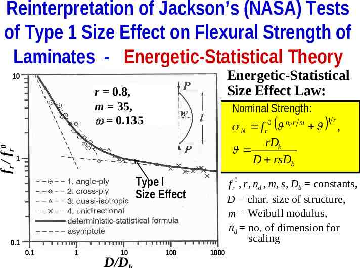
Reinterpretation of Jackson’s (NASA) Tests of Type 1 Size Effect on Flexural Strength of Laminates - Energetic-Statistical Theory Energetic-Statistical Size Effect Law: 10 fr / fr0 r 0.8, m 35, 0.135 Nominal Strength: 1r N f r0 nd r m , rDb D rsDb 1 Type I Size Effect f r0 , r , nd , m, s, Db constants, D char. size of structure, m Weibull modulus, nd no. of dimension for scaling 0.1 0.1 1 10 D/D 100 1000
Best Fits of Jackson’s (NASA) Individual Data Sets of Laminates Stat. Theory Alone m 3 m 30 Energetic Weibull theory m 3 and CoV 3 % ? Weibull theory m 30 and CoV 23 % ? Laminate stacking sequence: 1. angle-ply 2. cross-ply 3. quasi-isotropic 4. unidirectional
Optimum Fit of Existing Test Data Numerical Simulations by Nonlocal Weibull 4 TheoryNumerical : 4 3 Tests : 3 2 1 0.5 0.1 Statistical formula, m 24 asymptote-large n asymptote-small m 2 tr/tr, log(fr/fr, ) Nonlocal Weibull (III) 1 1 10 D/Db Db 100 1000 0.5 0.1 n m 1 log(D/Db) (Size) Nielson 1954 3 point Wright 1952 4 point Wright 1952 1inch Walker&Bloem 1957 2inch Walker&Bloem 1957 Reagel&Willis 1931 Sabnis&Mirza 1979 Rokugo 1995 Rocco 1995 Lindner 1956 Statistical formula, m 24 asymptote-small asymptote-large 10 D/Db 100 1000 D After Bazant, Xi, Novak (1991, 2000)
Nonlocal Weibull Theory (Bažant and Xi, 1991) way ave loc Nonlocal generalization (finite RVE): al spatial density of failure probability of continuum point rag ed Classical (local) theory: – weakest-link model if one RVE is a continuum point: to combine statistical & energetic size effects nonlocal strain over one RVE.
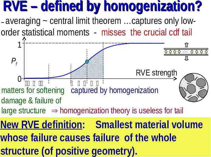
RVE – defined by homogenization? averaging central limit theorem captures only loworder statistical moments - misses the crucial cdf tail – 1 Pf RVE strength 0 matters for softening captured by homogenization damage & failure of large structure homogenization theory is useless for tail New RVE definition: Smallest material volume whose failure causes failure of the whole structure (of positive geometry).
Can RVE be largely or mostly Weibullian? NO! Proof: 1 Pf 0 RVE? NO! Assumed Weibull RVE strength Assume RVE to be largely Weibullian But then the RVE must behave as a chain But then damage must localize into one sub-RVE So the sub-RVE must be the true RVE This must be true RVE!
Chain of Gaussian RVEs – Gumbel 4 ln{ln[ 1/(1– Pf )]} 0 Present Theory -4 4 Weibull distribution (finite threshold) 3.5x 4 Pf 10-6 5 6 ln 7 10 104 5 Present Theory 0 -4 -1 2 3 4 Dental Ceramics Alumina-glass Composite 0 Neq 500 -8 Lohbauer et al. 2002 -1 2 -4 2 .6 0 ln( u) 4 8 Weibull distribution (finite threshold) 2 .4 105 104 Neq 500 -8 4 -4 -8 -1 2 ln(mean strength) ln{ln[ 1/(1– Pf )]} Comparison of Present Theory (No Threshold) to Weibull Model with Finite Threshold 5 Weibull distribution (finite threshold) 6 7 ln 2 .2 Present Theory (zero threshold) 2 4 1 ln( eq) m 6
Optimum Fit by Weibull Theory with Finite Threshold 3-pt Bend Test on Porcelain (Weibull 1939) u 13.4 16.4 S.F 1.22 ndata 102 ln{ ln[ 1/(1– Pf ) ] } Pf 10-1 10-2 10 -3 4-pt Bend Test on Dental Alumina-Glass Composite (Lohbauer et al., 2002) u 230 398 S.F 1.73 ndata 27 4.39 u 190 361 S.F 1.84 ndata 107 3.8 1 10-5 2.1 design 13.5 2.3 1 2 18.6mm 100mm 10-6 2.5 4 3 12.5 2.7 2.9 -4 design 230.1 12.5 20 0 4 3 8 4-pt Bend Test on Sintered Si3N4 with 4-pt Bend Test on Sintered Si3N4 with Y2O3/Al2O3 Additives CTR2O3/Al2O3 Additives (Santos et al., 2003) (Santos et al., 2003) u 586 691 S.F 1.18 ndata 27 -1 10-2 10 4-pt Bend Test on Sintered –SiC (Salem et al., 1996) 1.81 1 10-4 10 (incorrect) -3 u 577 662 S.F 1.15 ndata 21 2.7 1 10-4 1 design 196 2 6 3 8 4 6 5 6 4-pt Bend Test on Sintered Si3N4 (Gross, 2003) u 588 733 S.F 1.25 ndata 27 1.7 1 1.7 1 10-5 4 3 10-6 -2 design 586 0 10 2 20 10 4 4 3 -4 design -2 577 10 0 20 2 10 4 ln( u) -4 design 588 4 3. 1 10.4 0 10.4 19.6 4
Optimum Fit by Chain–of–RVEs, Zero Threshold 3-pt Bend Test, Porcelain ln{ ln[ 1/(1– Pf )]} 1 (correct) 4-pt Bend Test on Dental Alumina-Glass Composite 4-pt Bend Test, Sintered –SiC 2 2 Pf 0.80 0 0 0 ndata 102 Pf 0.40 Pf 0.20 -1 -2 -2 18.6mm 24 100mm 1 -3 16 8 -4 4 3 12.5 1 20 2.8 2.9 6 5.5 6 .5 4-pt Bend Test on Sintered Si3N4 with 4-pt Bend Test on Sintered Si3N4 with Y2O3/Al2O3 Additives CTR2O3/Al2O3 Additives 2.0 2 0 0.0 0 -2 Pf 0.25 -2.0 32 1 10 20 10 -4 6.4 6.5 6.6 6.7 -4.0 6.35 4 3 8 6 5.9 6.1 ndata 27 -2 30 10 20 1 10 -4 6.45 5.7 Pf 0.25 ndata 21 40 1 4 3 6 4-pt Bend Test on Sintered Si3N4 2 ndata 27 3 -6 5 .5 Pf 0.30 2 1 12.5 -4 2.7 ndata 107 -2 ndata 27 6.55 6.65 ln( ) (stress) 6.4 4. 3. 0 1 6.5 10.4 6.6 19.6 6.7 10.4 6.8
Optimum Fits by Chain-of-RVEs (zero threshold), Weibull cdf with Finite Threshold, and Gaussian cdf 4-pt Bend Test on Dental Alumina-Glass Composite 3-pt Bend Test on Porcelain ln{ln[1/(1– Pf )]} Pf 10-1 S.FG 1.30 S.FR 1.70 S.FW 1.22 4-pt Bend Test on Sintered –SiC S.FG 3.14 S.FR 2.12 S.FW 1.84 10-2 10-3 24 10-4 8 1 10-5 S.FG N.A. S.FR 5.53 S.FW 1.73 1 16 1 Chain-of-RVEs Asymptotic cdfs Gaussian cdf Weibull cdf, finite threshold 10-6 Pf 10-1 2.2 des,R 9.70 des,G 2.6 des,W 12.62 13.51 3.0 4 4-pt Bend Test on Sintered Si3N4 with Y2O3/Al2O3 Additives S.FG 1.53 S.FR 1.57 S.FW 1.18 des,W 68 des,R 230.1 5 6 4.5 7 4-pt Bend Test on Sintered Si3N4 with CTR2O3/Al2O3 Additives S.FG 1.55 S.FR 1.42 S.FW 1.15 des,G des,R des,W 5.5 115 170 196 4-pt Bend Test on Sintered Si3N4 S.FG 2.27 S.FR 1.75 S.FW 1.25 With Threshold (wrong) 10-2 10-3 32 10-4 44 1 Gaussian 1 10-5 30 1 10-6 6.0 des,R des,G des,W 6.4 440 453 587 ln 6.8 6.0 des,G des,R des,W 426 465 577 6.4 6.5 des,G 6.8 5.6 des,R des,W6.2 323 419 588 (strength in expanded scale) No Threshold (correct) 6.8
Lifetime
Lifetime cdf via Morse Interatomic Potential Mean time between interatomic scission under a constant stress: Unstressed and stressed energy well E ( ) 0 exp[Q( ) / kT ] Atomic vibration Nonl. stress dependence Period of activation energy barrier Morse interatomic potential for 1 bond: E (r ) Q0 [1 e a ( r r0 ) 2 ] Morse Potential bond d e s s e r t s Un St res Q0 se db on Q d Energy barrier as function of stress ) (Phoenix): Q Q ln( / 0 0 Failure probability of atomic lattice: d t F 1 exp 0 [ (t )] s log(Pf) Dissociation energy barrier Q0 s / kT 1 (1/s 10 to 50) Ftail 0 s 0 log( ) Q0 s kT r
Distribution of Lifetime for 1 RVE a) Series Coupling b) Parallel Coupling 1 2 N n Extent of power-law tail is shortened by parallel coupling: 12 If each link has tail m, the chain has the If each fiber has tail p, n 2: Ptail 10-3 10-2 same tail m the bundle has tail np n 3: P 10-5 10-4 tail additive exponents long chains c) Hierarchical Model of Lifetime Distribution Parallel coupling produces cdf with Gaussian core. Series coupling increases the power-tail reach. Power-law tail with zero threshold is indestructible!
Implications Implicationsfor forLifetime Lifetimecdf cdfat atMacro-Scale Macro-Scale 1) Weibull moduli for strength cdf ms and lifetime cdf m ms nQ0 s / kT n 1 m ns 2) Dependence of cdf of lifetime on structure size Pf 1 Neq 104 Neq 500 Weibull Neq 1 Gaussian ms Q0 m kT proportional to activation energy barrier 3) Size effect on mean structural lifetime log( ) ms/m 10 50 Much stronger size effect! Weibull asymptote 1 0 Increasing size Structural lifetime m log D (Size)
Failure probability distribution as a function of applied stress and load duration 1 Weibull 103 102 Grafted 10 / ref 1 Pf 0 . 5 /s0 0 1 0 1 2 Pf 3 Weibull Pf /s0 1.2 Grafted Weibull 1.1 0.95 Gaussian 0.8 0 .5 0 0 2 4 6 / log( / ref) s0 ) f e r / ( g lo
Effect of loading duration on mean structural strength µ 10 24 0 log( / 0 ) 6 10 3 10 2 -0 .2 -0 .3 / 10 ref 1 1 -0 .4 m 24 -0 .5 log( /µ0 ) 1 0 1 0 24 2 3 4 log(Neq) 10 3 50 1 50 10 Ne q 1 -0 .1 -0 .2 -0 .3 -0 .4 s 1/50 -0 .5 0 2 1 4 log(mean strength, µ) -0 .1 log(N eq ) 50 6 log( / ref) ) f / e r log(
Simple Probabilistic Analysis via Asymptotics
Type 1 Size Effect on Mean and Each RVE one hierarchical model Small (D 0) Small Size Asymptote Larger D Intermediate Asymptote Gaussian pdf Higher T Longer Weibull pdf log N ( Nom. Strength ) pdf via Asymptotic Matching l rn m rD N f r0 s b lo D ls D Large Size Asymptote m 1 r Large D nd D log D ( Size )
Malpasset Dam, failed 1959 —size effect must have contributed
Ruins of Malpasset Dam Failed 1959, at Frejus French Maritime Alps Photos by Hubert Chanson and Alain Pasquet
Cause of Failure of Malpasset Dam Sudden Localized Fracture Tolerable movement of abutment would today be 77% smaller.
Deterministic Computations by ATENA with Microplane Model for Scaled Dams of Various Sizes MODEL - progressive distributed cracking REAL - sudden localized fracture
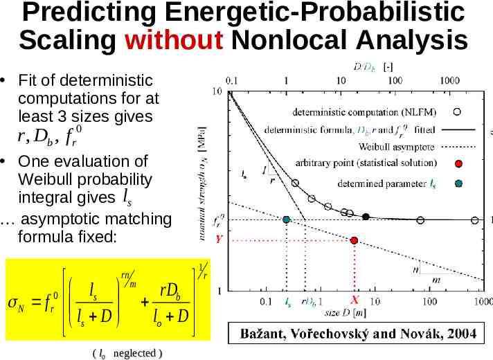
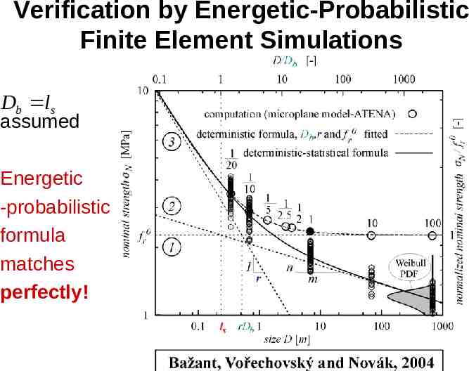
Predicting Energetic-Probabilistic Scaling without Nonlocal Analysis Fit of deterministic computations for at least 3 sizes gives r , Db , f r0 One evaluation of Weibull probability integral gives ls asymptotic matching formula fixed: l N f r0 s ls D rn lo 1 m rDb lo D ( l0 neglected ) r
Verification by Energetic-Probabilistic Finite Element Simulations Db ls assumed Energetic -probabilistic formula matches perfectly!
CONCLUSION For quasibrittle materials, not only the mean nominal strength, but also the strength distribution, the safety factors and lifetime distribution, depend on structure size and shape. Google “Bazant”, then download 455.pdf ,464.pdf, 465.pdf, 470.pdf .