GenomicSEM: A Novel Method for Modeling Multivariate Genetic

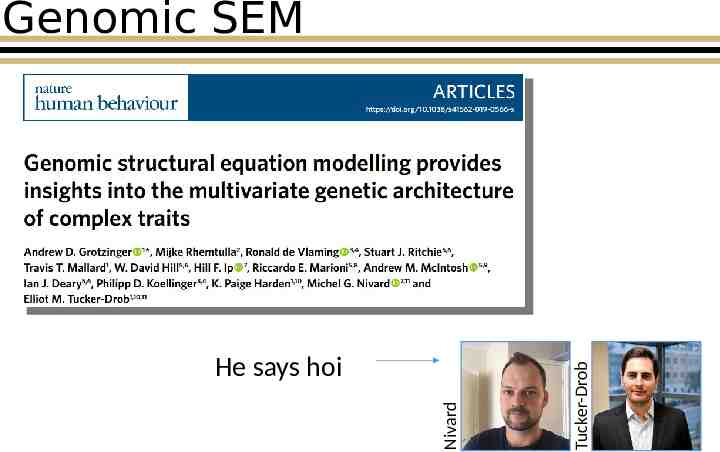
GenomicSEM: A Novel Method for Modeling Multivariate Genetic Architecture Presented by: Andrew D. Grotzinger Paper: Grotzinger, A. D., Rhemtulla, M., de Vlaming, R., Ritchie, S. J., Mallard, T. T., Hill, W. D, Ip, H. F., McIntosh, A. M., Deary, I. J., Koellinger, P. D., Harden, K. P., Nivard, M. G., & Tucker-Drob, E. M. (in press). Genomic SEM provides insights into the multivariate genetic architecture of complex traits. Nature Human Behaviour. Link to paper: rdcu.be/bvn7t

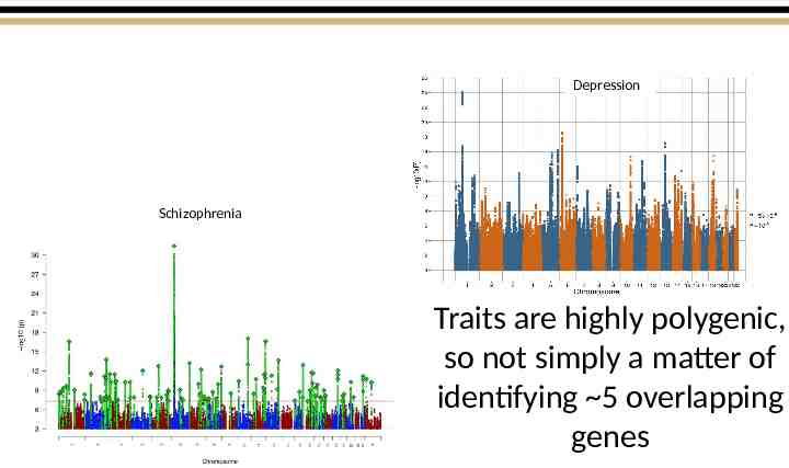
Depression Schizophrenia Traits are highly polygenic, so not simply a matter of identifying 5 overlapping genes

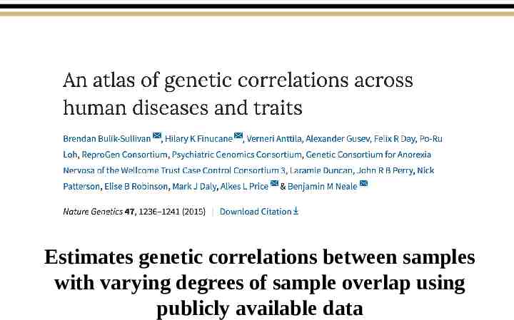
Estimates genetic correlations between samples with varying degrees of sample overlap using publicly available data

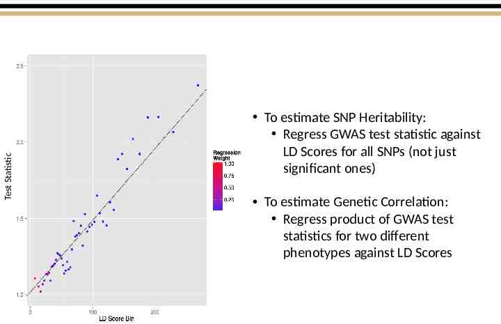
Test Statistic To estimate SNP Heritability: Regress GWAS test statistic against LD Scores for all SNPs (not just significant ones) To estimate Genetic Correlation: Regress product of GWAS test statistics for two different phenotypes against LD Scores

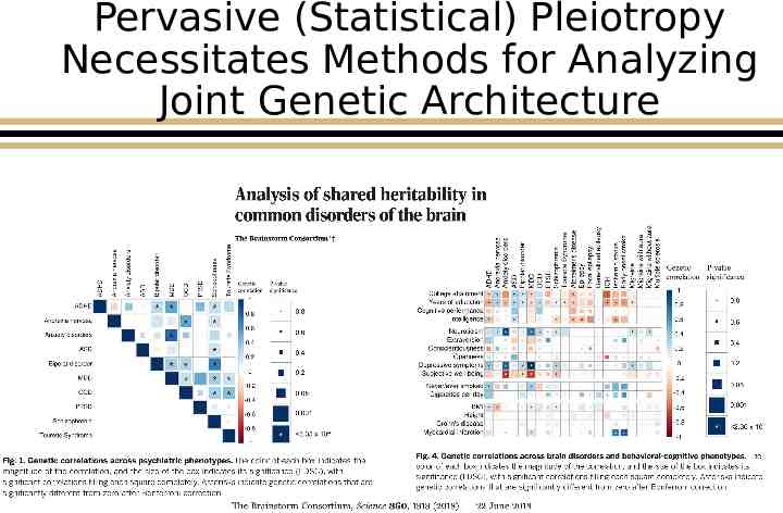
Pervasive (Statistical) Pleiotropy Necessitates Methods for Analyzing Joint Genetic Architecture

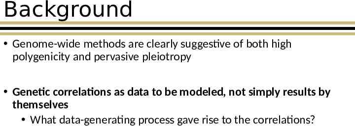
Background Genome-wide methods are clearly suggestive of both high polygenicity and pervasive pleiotropy Genetic correlations as data to be modeled, not simply results by themselves What data-generating process gave rise to the correlations?

Nivard He says hoi Tucker-Drob Genomic SEM

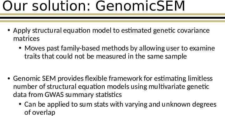
Our solution: GenomicSEM Apply structural equation model to estimated genetic covariance matrices Moves past family-based methods by allowing user to examine traits that could not be measured in the same sample Genomic SEM provides flexible framework for estimating limitless number of structural equation models using multivariate genetic data from GWAS summary statistics Can be applied to sum stats with varying and unknown degrees of overlap

Short Primer on Structural Equation Modeling (SEM)

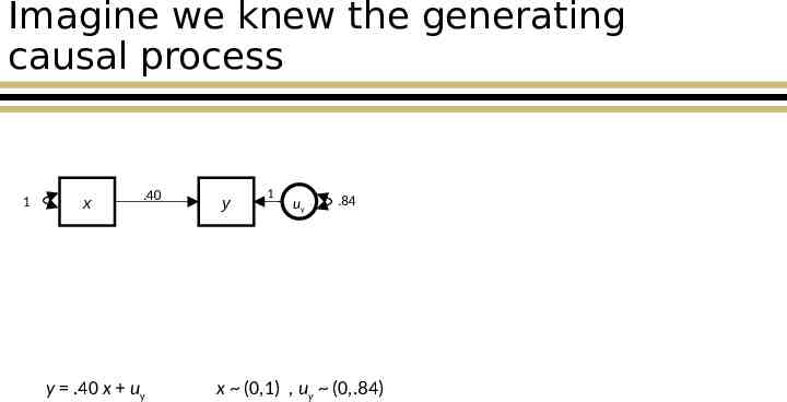
Imagine we knew the generating causal process 1 x .40 y .40 x uy y 1 uy .84 x (0,1) , uy (0,.84)

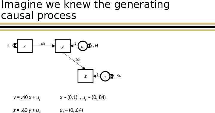
Imagine we knew the generating causal process 1 x .40 y 1 .84 uy .60 z 1 uz y .40 x uy x (0,1) , uy (0,.84) z .60 y uz uz (0,.64) .64

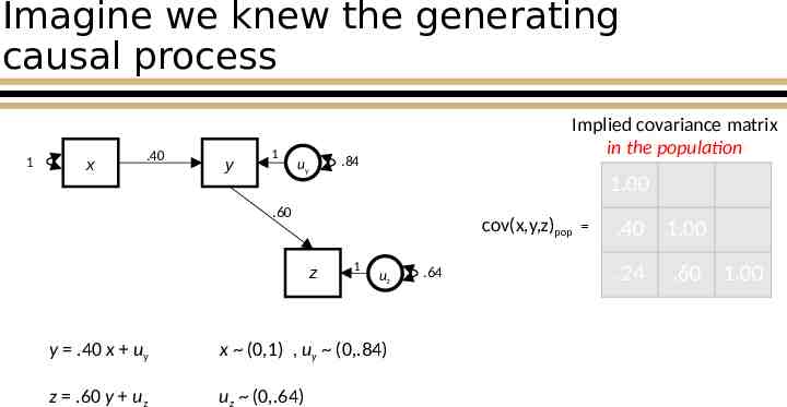
Imagine we knew the generating causal process 1 x .40 y 1 Implied covariance matrix in the population .84 uy 1.00 .60 cov(x,y,z)pop z 1 uz y .40 x uy x (0,1) , uy (0,.84) z .60 y uz uz (0,.64) .64 .40 1.00 .24 .60 1.00

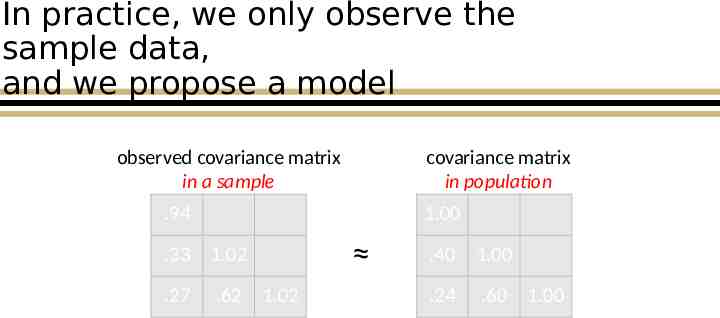
In practice, we only observe the sample data, and we propose a model covariance matrix in population observed covariance matrix in a sample .94 1.00 .33 1.02 .27 .62 1.02 .40 1.00 .24 .60 1.00

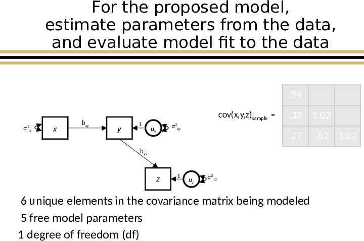
For the proposed model, estimate parameters from the data, and evaluate model fit to the data .94 σ2 x x bxy cov(x,y,z)sample y 1 .33 1.02 σ2uy uy .27 byz z 1 uz σ2uz 6 unique elements in the covariance matrix being modeled 5 free model parameters 1 degree of freedom (df) .62 1.02

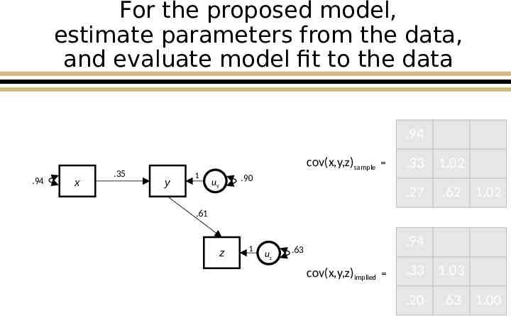
For the proposed model, estimate parameters from the data, and evaluate model fit to the data .94 .94 x .35 cov(x,y,z)sample y 1 .33 1.02 .90 uy .27 .62 1.02 .61 z 1 uz .94 .63 cov(x,y,z)implied .33 1.03 .20 .63 1.00

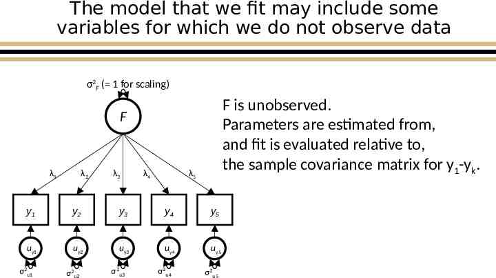
The model that we fit may include some variables for which we do not observe data σ2F ( 1 for scaling) F is unobserved. Parameters are estimated from, and fit is evaluated relative to, the sample covariance matrix for y1-yk. F λ1 λ2 λ3 λ4 λ5 y1 y2 y3 y4 y5 uy1 uy2 uy3 uy4 uy5 σ2u1 σ2u2 σ2u3 σ2u4 σ2u5

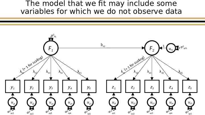
The model that we fit may include some variables for which we do not observe data σ2F1 b12 F1 ( λ11 for 1 ing l a sc λ12 F2 ) li sca λ13 λ14 for 1 λ21( λ22 λ15 ng 1 uF1 σ2uF1 ) λ23 λ24 λ25 y1 y2 y3 y4 y5 z1 z2 z3 z4 z5 uy1 uy2 uy3 uy4 uy5 uz1 uz2 uz3 uz4 uz5 σ2uy4 σ2uy5 σ2uz4 σ2uz5 σ2uy1 σ2uy2 σ2uy3 σ2uz1 σ2uz2 σ2uz3

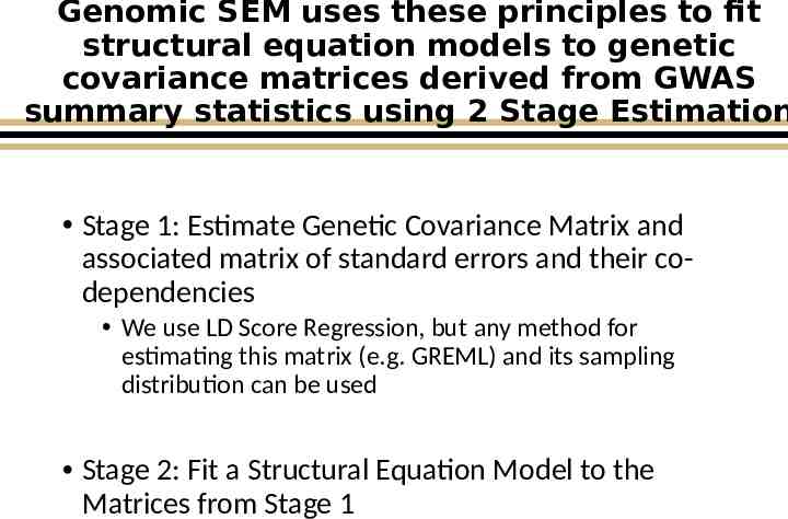
Genomic SEM uses these principles to fit structural equation models to genetic covariance matrices derived from GWAS summary statistics using 2 Stage Estimation Stage 1: Estimate Genetic Covariance Matrix and associated matrix of standard errors and their codependencies We use LD Score Regression, but any method for estimating this matrix (e.g. GREML) and its sampling distribution can be used Stage 2: Fit a Structural Equation Model to the Matrices from Stage 1

Fitting Structural Equation Models to GWAS-Derived Genetic Covariance Matrices

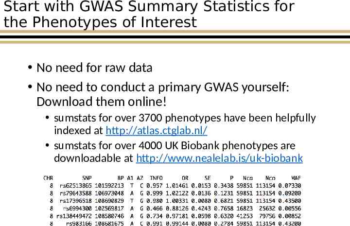
Start with GWAS Summary Statistics for the Phenotypes of Interest No need for raw data No need to conduct a primary GWAS yourself: Download them online! sumstats for over 3700 phenotypes have been helpfully indexed at http://atlas.ctglab.nl/ sumstats for over 4000 UK Biobank phenotypes are downloadable at http://www.nealelab.is/uk-biobank

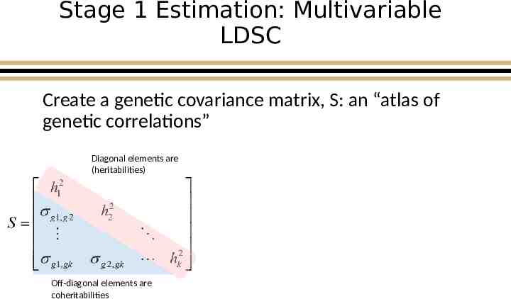
Stage 1 Estimation: Multivariable LDSC Create a genetic covariance matrix, S: an “atlas of genetic correlations” Diagonal elements are (heritabilities) Off-diagonal elements are coheritabilities

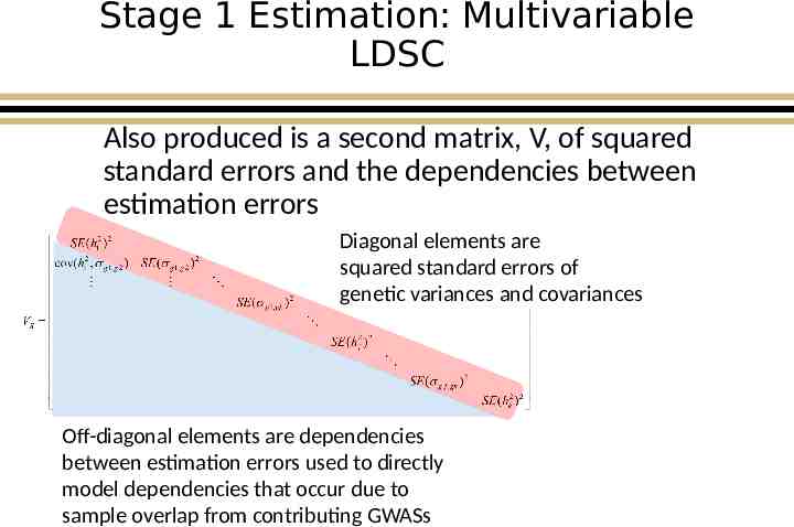
Stage 1 Estimation: Multivariable LDSC Also produced is a second matrix, V, of squared standard errors and the dependencies between estimation errors Diagonal elements are squared standard errors of genetic variances and covariances Off-diagonal elements are dependencies between estimation errors used to directly model dependencies that occur due to sample overlap from contributing GWASs

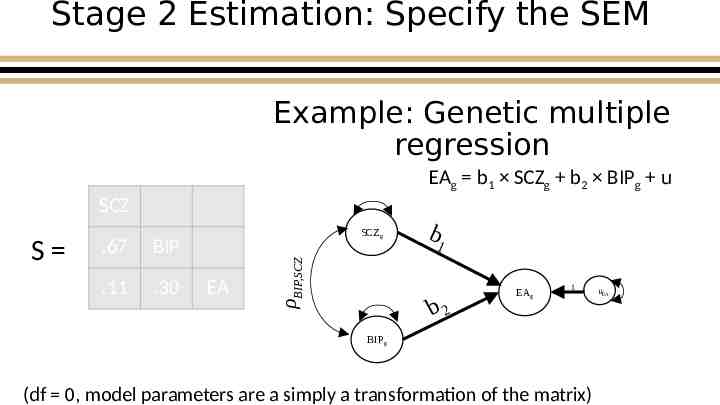
Stage 2 Estimation: Specify the SEM Example: Genetic multiple regression EAg b1 SCZg b2 BIPg u SCZ BIP .11 .30 EA ρBIP,SCZ S .67 SCZg b1 b2 EAg 1 BIPg (df 0, model parameters are a simply a transformation of the matrix) uEA

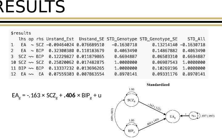
RESULTS EAg -.163 SCZg .406 BIPg u

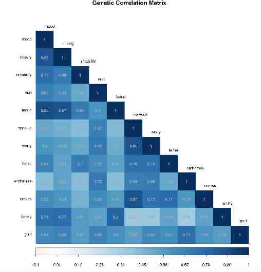
Example 2: Model Comparisons for Neuroticism 12 neuroticism traits from round 1 of Neale Lab UKB GWAS Goal use model fit indices to compare common factor, two-factor, and three-factor model

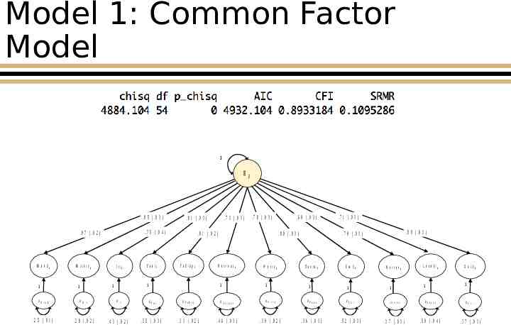
Model 1: Common Factor Model .2 7 ( .0 1 ) .2 6 ( .0 1 ) .2 9 ( .0 1 ) M ood M is e ry g g 1 u .2 2 ( .0 1 ) N e rv o u sg W o rry u Irr u Feel u F ed -up .0 3 ( .0 1 ) .0 5 ( .0 1 ) .0 4 (.0 1 ) .0 4 ( .0 1 ) u u Em bg 1 .2 4 ( .0 1 ) L o n e ly N erv e sg 1 uEm .0 5 ( .0 1 ) .0 5 ( .0 1 ) b G u iltg g 1 1 1 u Tense W o rry .0 5 ( .0 1 ) 0 5 (.0 1 ) b Tenseg g 1 N e rv o u s .2 0 ( .0 1 ) .2 4 ( .0 1 ) .2 8 ( .0 1 ) 1 M is M ood .0 3 ( .0 1 ) F e d -u p G 1 1 .2 8 (.0 1 ) .2 6 ( .0 1 ) .2 7 ( .0 1 ) F e e lG Irrg 1 u .2 5 ( .0 1 ) u uN erves .0 3 ( .0 1 ) u L o n e ly .0 4 ( .0 1 ) G u ilt .0 3 ( .0 1 ) S ta n d a r d iz ed 1 N .8 5 ( .0 3 ) .7 5 ( .0 4 ) .8 7 ( .0 2 ) M ood g 1 uM M is e ry g ood .2 5 (.0 1 ) Irrg u F e e lG M is u Irr .2 8 (.0 2 ) .4 3 ( .0 2 ) .7 3 ( .0 3 ) Feel .3 5 ( .0 3 ) .6 9 (.0 3 ) F e d -u p G N e rv o u sg u F e d -u p .3 3 (.0 2 ) u W o rry g Tenseg 1 N e rv o u s .4 6 ( .0 3 ) u 1 W o rry .3 9 ( .0 2 ) .7 1 (.0 3 ) .8 0 ( .0 3 ) .7 9 ( .0 3 ) .8 0 ( .0 3 ) 1 u .7 8 ( .0 3 ) .8 1 (.0 2 ) 1 1 1 .8 1 ( .0 3 ) g u Ten se .3 6 ( .0 3 ) Em bg 1 uEm L o n e ly g G u iltg 1 1 u N erv e s u L o n ely u .3 7 (.0 3 ) .5 0 (.0 4 ) N e rv e sg 1 b .5 2 (.0 3 ) G u ilt .3 7 ( .0 3 )

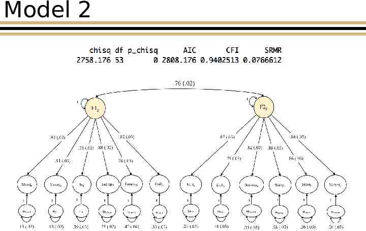
Model 2

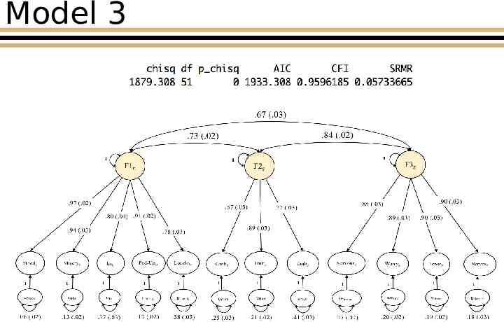
Model 3

Comparison of Model Fit Indices BUT Model 3 fits the best for CFI, SRMR and AIC Model 2 fits better than Model 1 Model 1 does OK .

Incorporating Genetic Covariance Structure into Multivariate GWAS Discovery

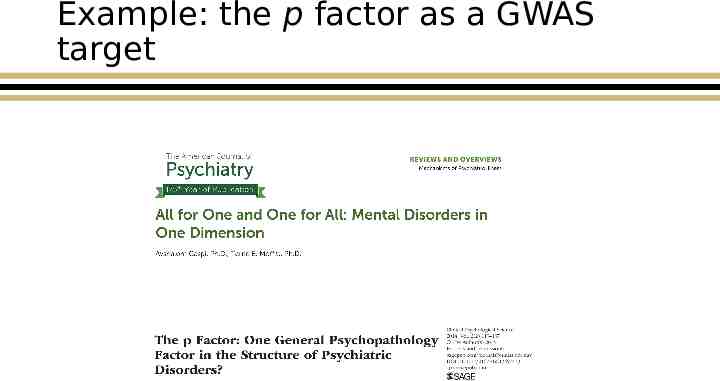
Example: the p factor as a GWAS target

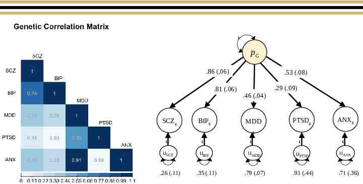
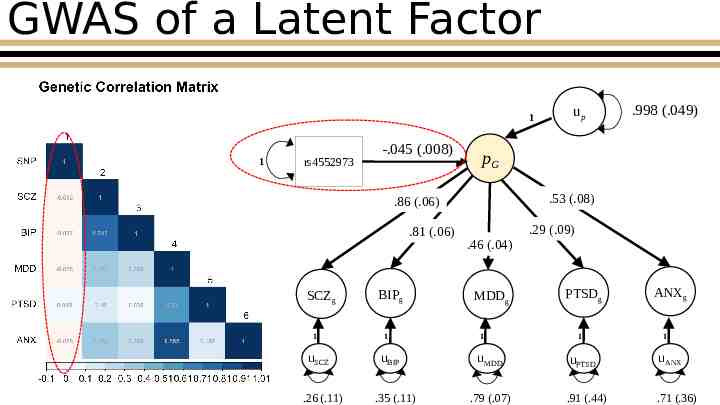
1 pG .86 (.06) .81 (.06) SCZg BIPg .53 (.08) .29 (.09) .46 (.04) MDD PTSDg ANXg g 1 uSCZ .26 (.11) 1 uBIP .35 (.11) 1 1 uMDD uPTSD .79 (.07) .91 (.44) 1 uANX .71 (.36)

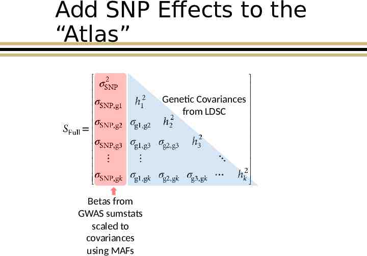
Add SNP Effects to the “Atlas” Genetic Covariances from LDSC Betas from GWAS sumstats scaled to covariances using MAFs

GWAS of a Latent Factor 1 1 rs4552973 -.045 (.008) SCZg 1 uSCZ .26 (.11) BIPg 1 uBIP .35 (.11) .998 (.049) pG .53 (.08) .86 (.06) .81 (.06) up .29 (.09) .46 (.04) MDDg 1 uMDD .79 (.07) PTSDg 1 ANXg 1 uPTSD uANX .91 (.44) .71 (.36)

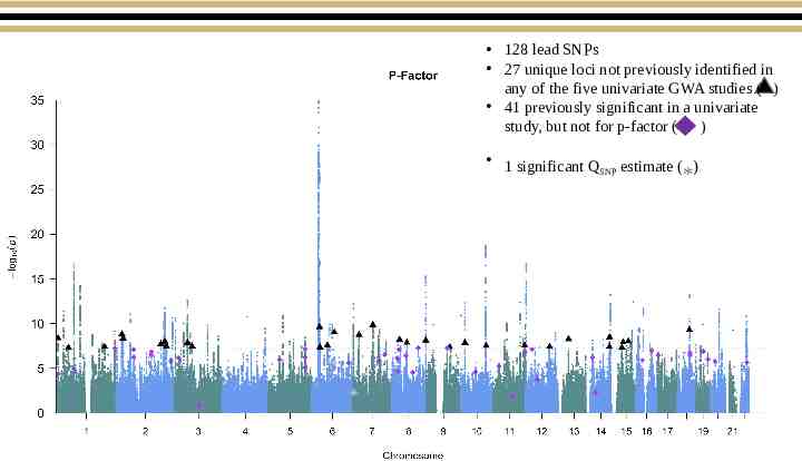
128 lead SNPs 27 unique loci not previously identified in any of the five univariate GWA studies ( ) 41 previously significant in a univariate study, but not for p-factor ( ) 1 significant Q estimate ( ) SNP *

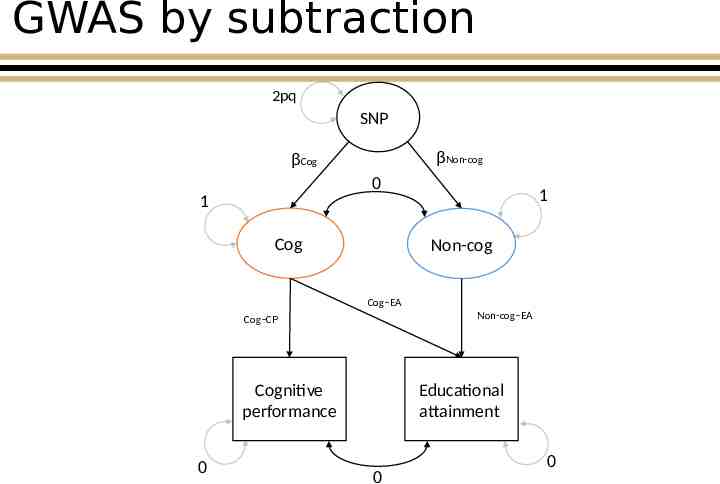
GWAS by subtraction 2pq SNP βNon-cog βCog 0 1 1 Cog Non-cog Cog–EA Non-cog–EA Cog–CP Cognitive performance 0 Educational attainment 0 0

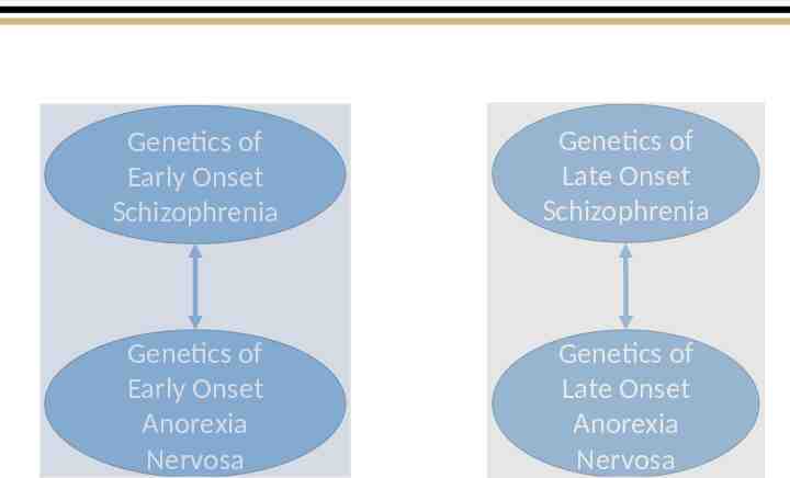
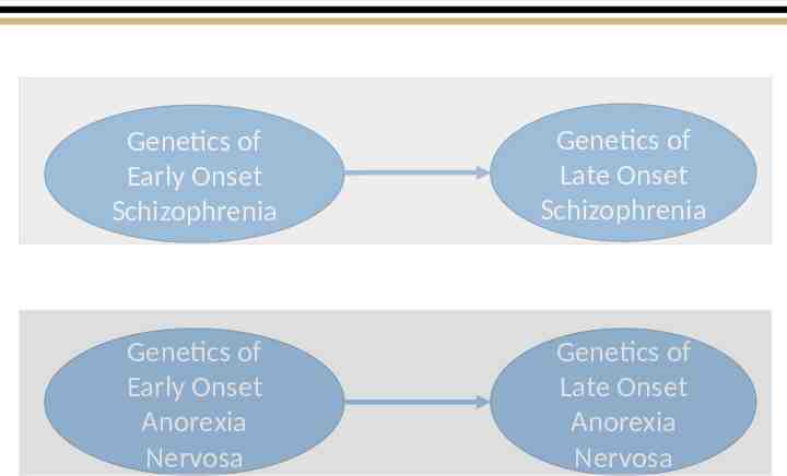
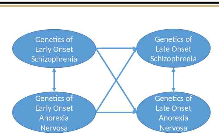
Even if you are not interested in genetics: Can now examine systems of relationships between a wide array of (rare) traits that could not be measured in the same sample

Genetics of Early Onset Schizophrenia Genetics of Late Onset Schizophrenia Genetics of Early Onset Anorexia Nervosa Genetics of Late Onset Anorexia Nervosa

Genetics of Early Onset Schizophrenia Genetics of Late Onset Schizophrenia Genetics of Early Onset Anorexia Nervosa Genetics of Late Onset Anorexia Nervosa

Genetics of Early Onset Schizophrenia Genetics of Late Onset Schizophrenia Genetics of Early Onset Anorexia Nervosa Genetics of Late Onset Anorexia Nervosa

Genetics of Early Onset Schizophrenia Genetics of Late Onset Schizophrenia Genetics of Early Onset Anorexia Nervosa Genetics of Late Onset Anorexia Nervosa

Practical

Practical outline I. II. III. IV. Initial considerations Estimating common factor models Estimating user specified model Estimating multivariate GWAS in Genomic SEM

I. Initial Considerations

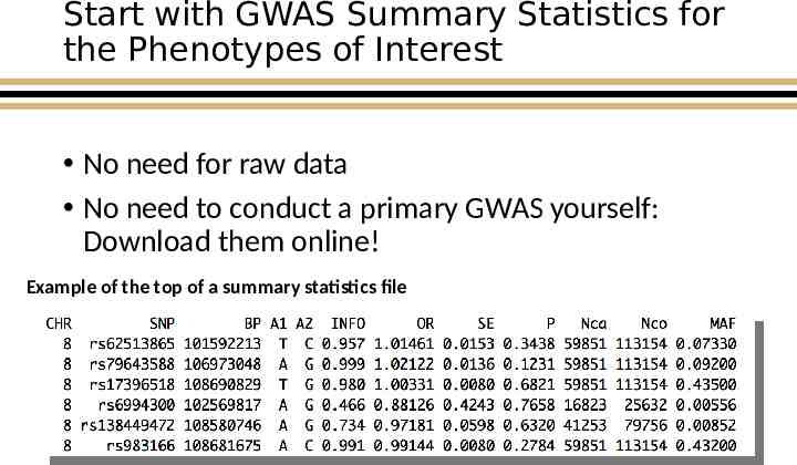
Start with GWAS Summary Statistics for the Phenotypes of Interest No need for raw data No need to conduct a primary GWAS yourself: Download them online! Example of the top of a summary statistics file

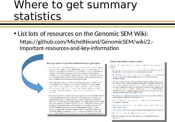
Where to get summary statistics List lots of resources on the Genomic SEM Wiki: https://github.com/MichelNivard/GenomicSEM/wiki/2.Important-resources-and-key-information

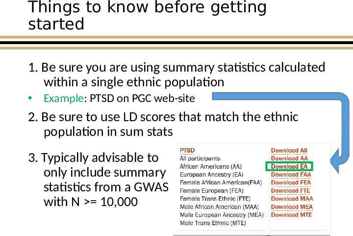
Things to know before getting started 1. Be sure you are using summary statistics calculated within a single ethnic population Example: PTSD on PGC web-site 2. Be sure to use LD scores that match the ethnic population in sum stats 3. Typically advisable to only include summary statistics from a GWAS with N 10,000

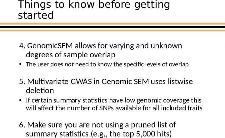
Things to know before getting started 4. GenomicSEM allows for varying and unknown degrees of sample overlap The user does not need to know the specific levels of overlap 5. Multivariate GWAS in Genomic SEM uses listwise deletion If certain summary statistics have low genomic coverage this will affect the number of SNPs available for all included traits 6. Make sure you are not using a pruned list of summary statistics (e.g., the top 5,000 hits)

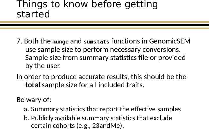
Things to know before getting started 7. Both the munge and sumstats functions in GenomicSEM use sample size to perform necessary conversions. Sample size from summary statistics file or provided by the user. In order to produce accurate results, this should be the total sample size for all included traits. Be wary of: a. Summary statistics that report the effective samples b. Publicly available summary statistics that exclude certain cohorts (e.g., 23andMe).

II. Estimating Common Factor Models in Genomic SEM

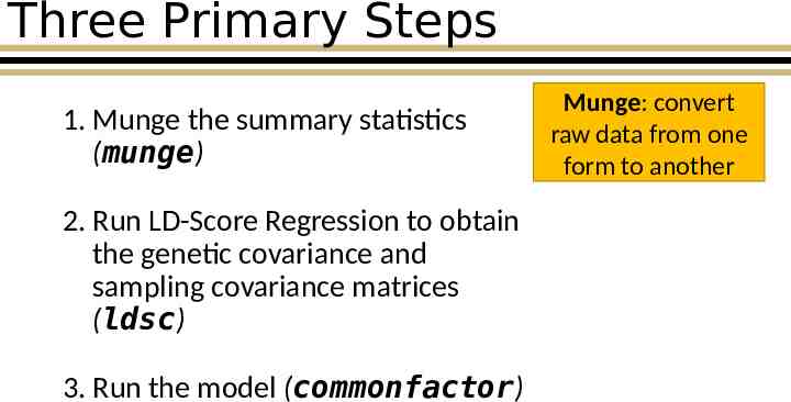
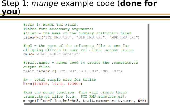
Three Primary Steps 1. Munge the summary statistics (munge) 2. Run LD-Score Regression to obtain the genetic covariance and sampling covariance matrices (ldsc) 3. Run the model (commonfactor) Munge: convert raw data from one form to another

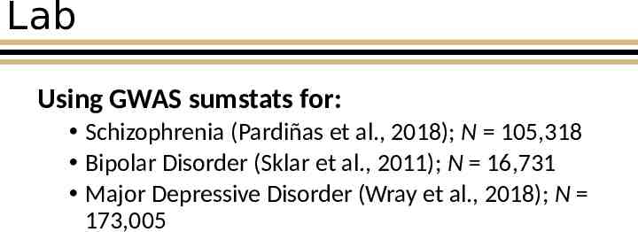
Lab Using GWAS sumstats for: Schizophrenia (Pardiñas et al., 2018); N 105,318 Bipolar Disorder (Sklar et al., 2011); N 16,731 Major Depressive Disorder (Wray et al., 2018); N 173,005

Step 1: munge example code (done for you)

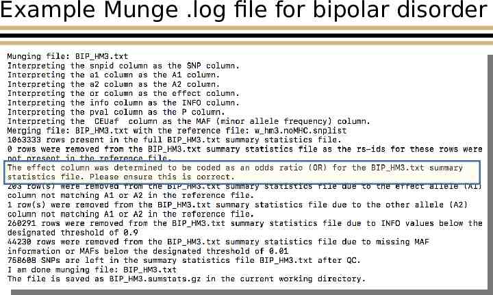
Example Munge .log file for bipolar disorder

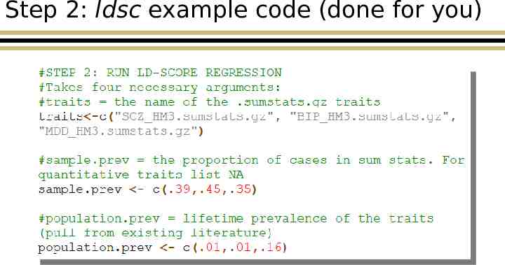
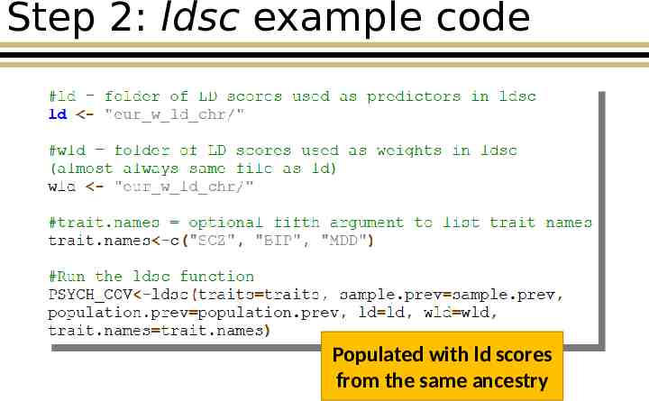
Step 2: ldsc example code (done for you)

Step 2: ldsc example code Populated with ld scores from the same ancestry

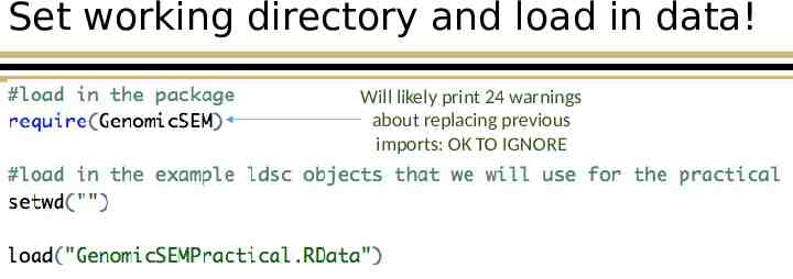
Set working directory and load in data! Will likely print 24 warnings about replacing previous imports: OK TO IGNORE

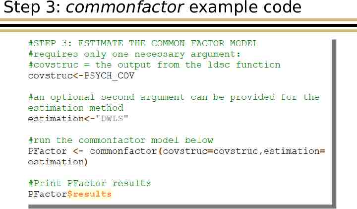
Step 3: commonfactor example code

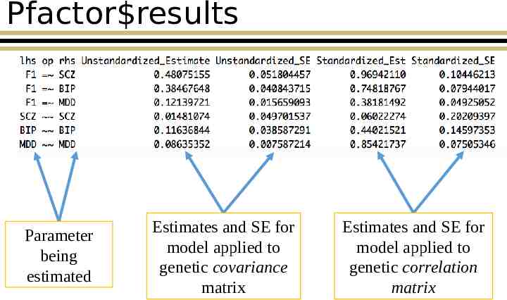
Pfactor results Parameter being estimated Estimates and SE for model applied to genetic covariance matrix Estimates and SE for model applied to genetic correlation matrix

III. Estimate a UserSpecified Model

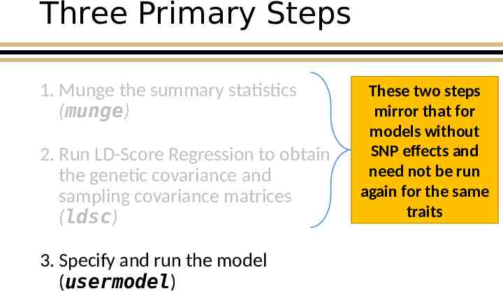
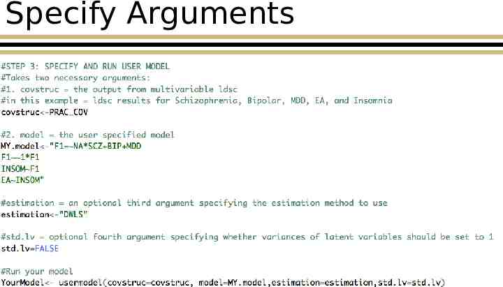
Three Primary Steps 1. Munge the summary statistics (munge) 2. Run LD-Score Regression to obtain the genetic covariance and sampling covariance matrices (ldsc) 3. Specify and run the model (usermodel) These two steps mirror that for models without SNP effects and need not be run again for the same traits

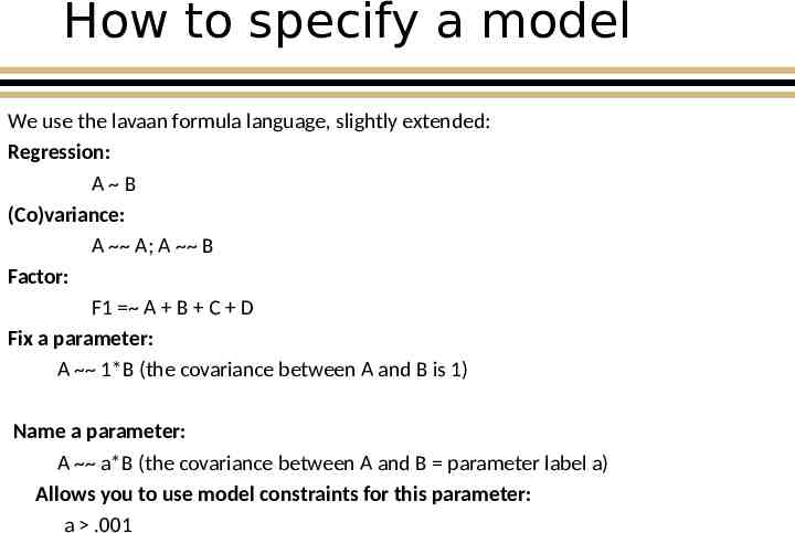
How to specify a model We use the lavaan formula language, slightly extended: Regression: A B (Co)variance: A A; A B Factor: F1 A B C D Fix a parameter: A 1*B (the covariance between A and B is 1) Name a parameter: A a*B (the covariance between A and B parameter label a) Allows you to use model constraints for this parameter: a .001

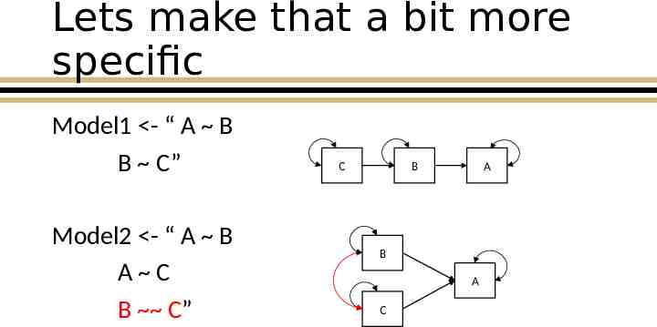
Lets make that a bit more specific Model1 - “ A B B C” Model2 - “ A B A C B C” C B A B A C

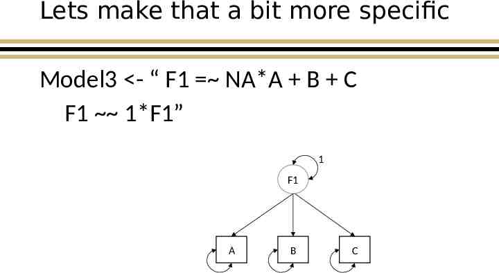
Lets make that a bit more specific Model3 - “ F1 NA*A B C F1 1*F1” 1 F1 A B C

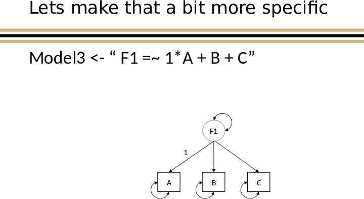
Lets make that a bit more specific Model3 - “ F1 1*A B C” F1 1 A B C

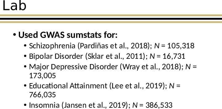
Lab Used GWAS sumstats for: Schizophrenia (Pardiñas et al., 2018); N 105,318 Bipolar Disorder (Sklar et al., 2011); N 16,731 Major Depressive Disorder (Wray et al., 2018); N 173,005 Educational Attainment (Lee et al., 2019); N 766,035 Insomnia (Jansen et al., 2019); N 386,533

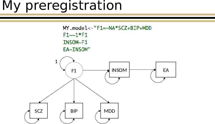
My preregistration 1 F1 SCZ BIP INSOM MDD EA

Specify Arguments

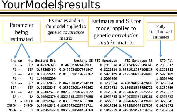
YourModel results Parameter being estimated Estimates and SE for model applied to genetic covariance matrix Estimates and SE for model applied to genetic correlation matrix matrix Fully standardized estimates

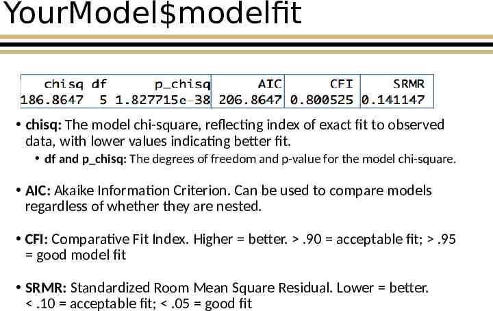
YourModel modelfit chisq: The model chi-square, reflecting index of exact fit to observed data, with lower values indicating better fit. df and p chisq: The degrees of freedom and p-value for the model chi-square. AIC: Akaike Information Criterion. Can be used to compare models regardless of whether they are nested. CFI: Comparative Fit Index. Higher better. .90 acceptable fit; .95 good model fit SRMR: Standardized Room Mean Square Residual. Lower better. .10 acceptable fit; .05 good fit

Delete Input for MY.model and run your own!

PRACTICAL: You Take Control As away of preregistering them, write your model down on paper Remember five variable names are: SCZ, BIP, MDD, EA, INSOM

IV. Multivariate GWAS in Genomic SEM

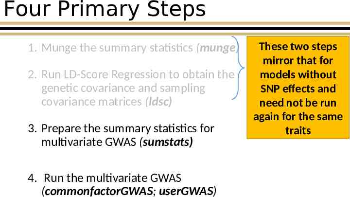
Four Primary Steps 1. Munge the summary statistics (munge) 2. Run LD-Score Regression to obtain the genetic covariance and sampling covariance matrices (ldsc) 3. Prepare the summary statistics for multivariate GWAS (sumstats) 4. Run the multivariate GWAS (commonfactorGWAS; userGWAS) These two steps mirror that for models without SNP effects and need not be run again for the same traits

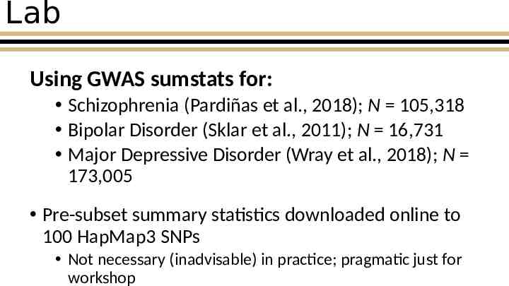
Lab Using GWAS sumstats for: Schizophrenia (Pardiñas et al., 2018); N 105,318 Bipolar Disorder (Sklar et al., 2011); N 16,731 Major Depressive Disorder (Wray et al., 2018); N 173,005 Pre-subset summary statistics downloaded online to 100 HapMap3 SNPs Not necessary (inadvisable) in practice; pragmatic just for workshop

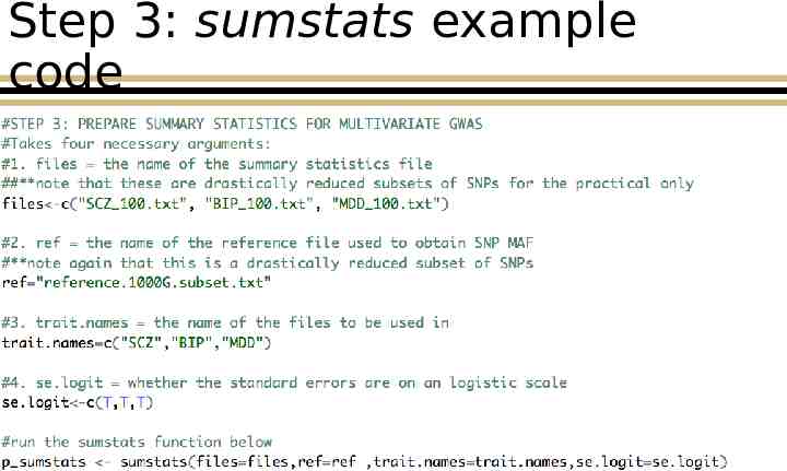
Step 3: sumstats example code

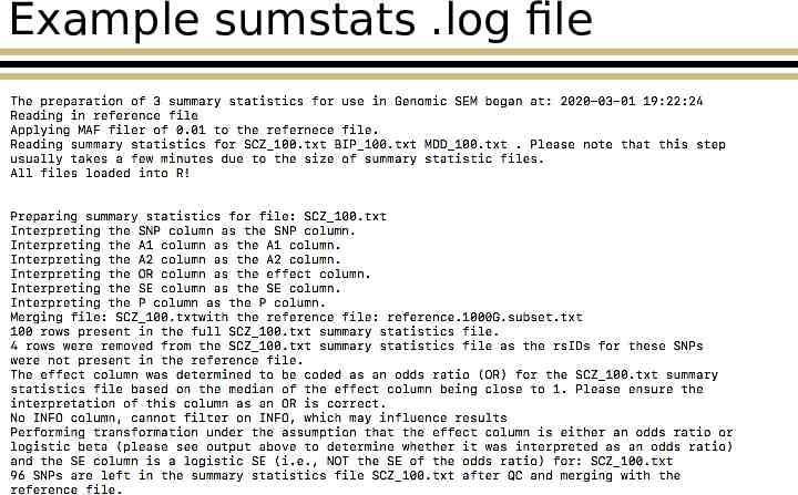
Example sumstats .log file

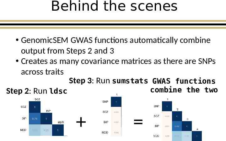
Behind the scenes GenomicSEM GWAS functions automatically combine output from Steps 2 and 3 Creates as many covariance matrices as there are SNPs across traits Step 3: Run sumstats GWAS functions combine the two Step 2: Run ldsc

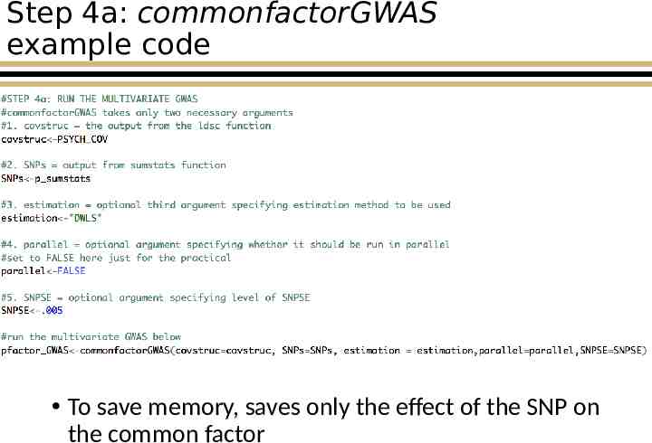
Step 4a: commonfactorGWAS example code To save memory, saves only the effect of the SNP on the common factor

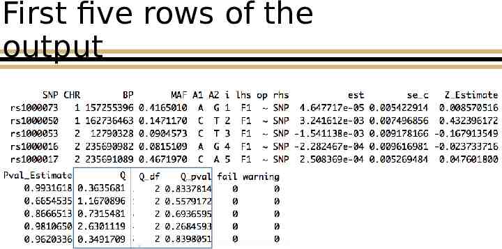
First five rows of the output

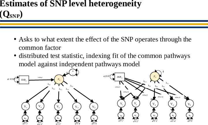
Estimates of SNP level heterogeneity (QSNP) Asks to what extent the effect of the SNP operates through the common factor distributed test statistic, indexing fit of the common pathways model against independent pathways model 1 𝜎 SNP 2 SNPm,F u 1 F 𝜎 SNP FG SNPm λV5 λV3 FG SNPm λV1 λV1 λV2 2 λV4 λV5 λV2 SNPm,V1 λV3 λV4 SNPm,V2 SNPm,V3 SNPm,V4 V1 V2 V3 V4 V5 g g g g g 11 1 1 1 1 uV uV uV 1 2 𝑒 V 12 𝑒V 2 2 3 𝑒 V 32 uV 4 𝑒V 42 uV 𝑒5 V 52 V1 V2 g 1 uV 1 𝑒 V 12 SNPm,V5 V3 V4 V5 g g g g 1 1 uV 2 𝑒 V 22 uV 3 𝑒V 3 2 1 1 uV uV 4 𝑒 V 42 5 𝑒V 52

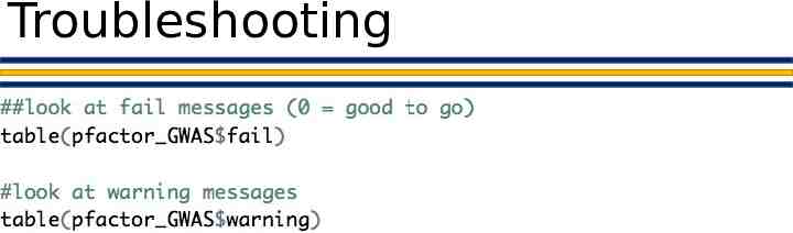
Troubleshooting

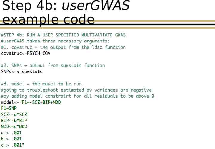
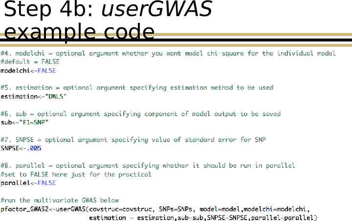
Step 4b: userGWAS example code

Step 4b: userGWAS example code

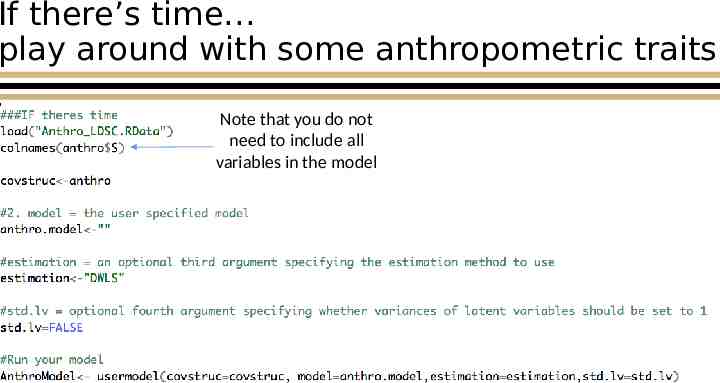
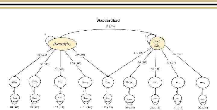
If there’s time play around with some anthropometric traits Note that you do not need to include all variables in the model

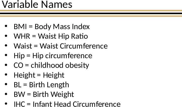
Variable Names BMI Body Mass Index WHR Waist Hip Ratio Waist Waist Circumference Hip Hip circumference CO childhood obesity Height Height BL Birth Length BW Birth Weight IHC Infant Head Circumference

Final Notes Parallel processing for both userGWAS and commonfactorGWAS is available Parallel is the same as serial processing, except that it takes an additional cores argument specifying how many cores to use Ideal run-time scenario: split jobs across computing nodes on a cluster and run in-parallel All runs are independent of one another!

Overview Genomic SEM is ready for use today! Ask questions on our google forum https://groups.google.com/forum/#!forum/genomic-sem-users Lots can be done using existing, openly available GWAS summary statistics Models are flexible and up to the user Use Genomic SEM to derive sumstats for novel phenotypes for use in PGS analyses

Resources See paper at: rdcu.be/bvn7t See github at: https://github.com/MichelNivard/GenomicSEM See tutorials at: https://github.com/MichelNivard/GenomicSEM/wi ki

Acknowledgements Elliot M. Tucker-Drob, Michel G. Nivard, Mijke Rhemtulla NIH grants R01HD083613, R01AG054628, R21HD081437, R24HD042849 Jacobs Foundation Royal Netherlands Academy of Science Professor Award PAH/6635 ZonMw grants 531003014, 849200011 European Union Seventh Framework Program (FP7/20072013) ACTION Project MRC grant MR/K026992/1 AgeUK Disconnected Mind Project