Multiple Regression

25 Slides281.00 KB
Multiple Regression
Introduction In this chapter, we extend the simple linear regression model. Any number of independent variables is now allowed. We wish to build a model that fits the data better than the simple linear regression model.
Computer printout is used to help us: – Assess/Validate the model How well does it fit the data? Is it useful? Are any of the required conditions violated? – Apply the model Interpreting the coefficients Estimating the expected value of the dependent variable
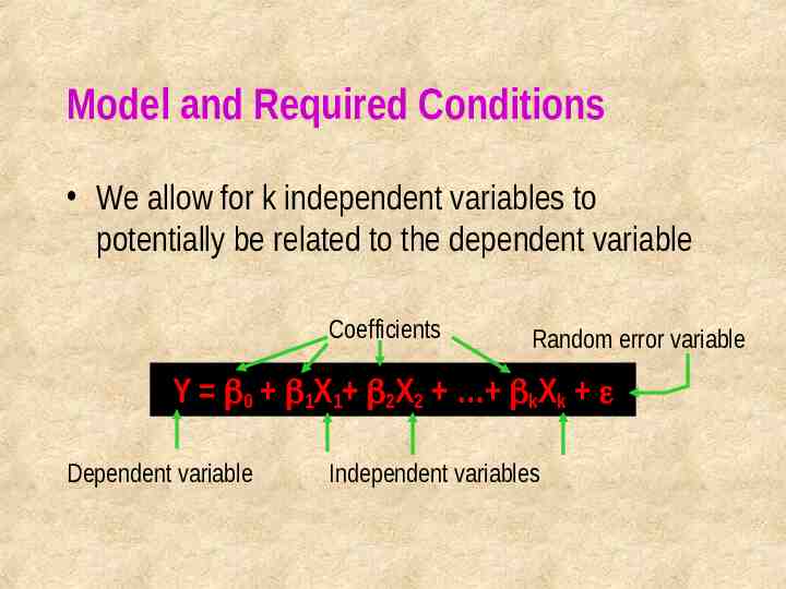
Model and Required Conditions We allow for k independent variables to potentially be related to the dependent variable Coefficients Random error variable Y 0 1X1 2X2 kXk Dependent variable Independent variables
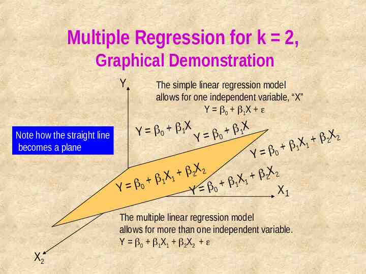
Multiple Regression for k 2, Graphical Demonstration Y Note how the straight line becomes a plane The simple linear regression model allows for one independent variable, “X” Y 0 1X X Y 0 1 Y X 1 0 0 Y X 2 2 X1 2X 2 X2 2 X 1 X 1 1 1 0 Y X1 Y 0 The multiple linear regression model allows for more than one independent variable. Y 0 1X1 2X2 X2 1
Required Conditions for the Error Variable The error is normally distributed. The mean is equal to zero and the standard deviation is constant ( for all possible values of the Xis. All errors are independent.
Estimating the Coefficients and Assessing the Model The procedure used to perform regression analysis: – Obtain the model coefficients and statistics using Excel. – Diagnose violations of required conditions. Try to remedy problems when identified. – Assess the model fit using statistics obtained from the sample. – If the model assessment indicates good fit to the data, use it to interpret the coefficients and generate predictions.
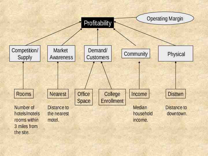
Example 18.1 Where to locate a new motor inn? – La Quinta Motor Inns is planning an expansion. – Management wishes to predict which sites are likely to be profitable, defined as having 50% or higher operating margin (net profit expressed as a percentage of total revenue). – Several potential predictors of profitability are: Competition (room supply) Market awareness (competing motel) Demand generators (office and college) Demographics (household income) Physical quality/location (distance to downtown)
Profitability Competition/ Supply Rooms Number of hotels/motels rooms within 3 miles from the site. Market Awareness Nearest Distance to the nearest motel. Demand/ Customers Office Space College Enrollment Operating Margin Community Physical Income Disttwn Median household income. Distance to downtown.
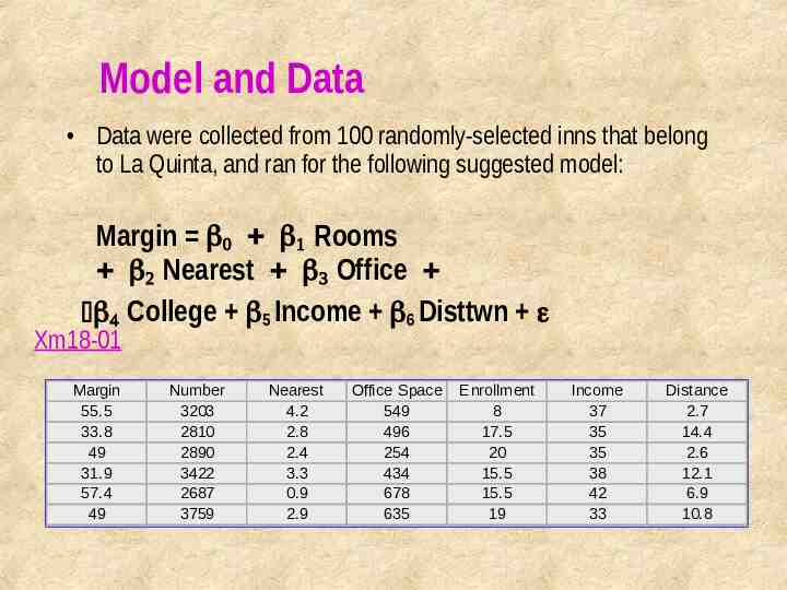
Model and Data Data were collected from 100 randomly-selected inns that belong to La Quinta, and ran for the following suggested model: Margin Rooms Nearest Office College 5 Income 6 Disttwn Xm18-01 Margin 55.5 33.8 49 31.9 57.4 49 Number 3203 2810 2890 3422 2687 3759 Nearest 4.2 2.8 2.4 3.3 0.9 2.9 Office Space 549 496 254 434 678 635 Enrollment 8 17.5 20 15.5 15.5 19 Income 37 35 35 38 42 33 Distance 2.7 14.4 2.6 12.1 6.9 10.8
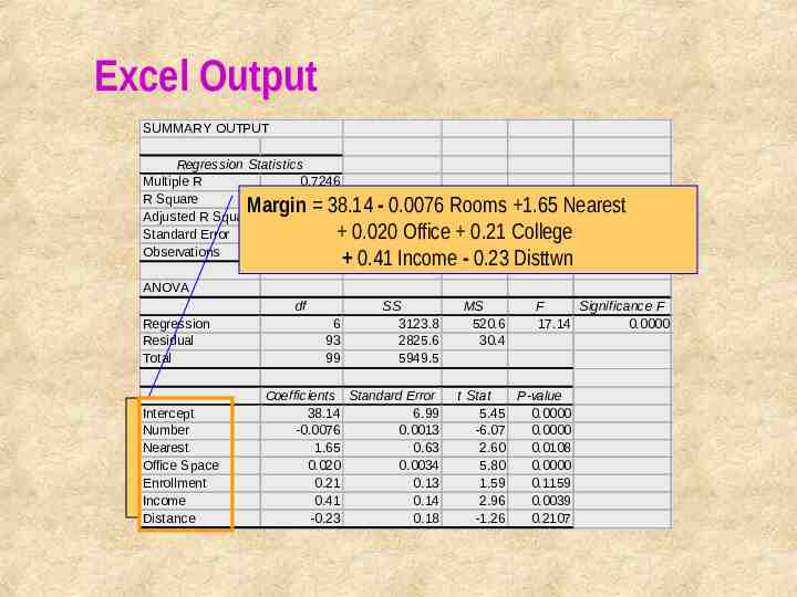
Excel Output SUMMARY OUTPUT Thisisisthe thesample sampleregression regressionequation equation This Regression Statistics (sometimes calledthe theprediction predictionequation) equation) (sometimes called Multiple R 0.7246 R Square 0.5251 Margin 38.14 - 0.0076 Rooms 1.65 Nearest Adjusted R Square 0.4944 Standard Error 5.51 0.020 Office 0.21 College Observations 100 0.41 Income - 0.23 Disttwn ANOVA df Regression Residual Total Intercept Number Nearest Office Space Enrollment Income Distance 6 93 99 SS 3123.8 2825.6 5949.5 Coefficients Standard Error 38.14 6.99 -0.0076 0.0013 1.65 0.63 0.020 0.0034 0.21 0.13 0.41 0.14 -0.23 0.18 MS 520.6 30.4 F Significance F 17.14 0.0000 t Stat P-value 5.45 0.0000 -6.07 0.0000 2.60 0.0108 5.80 0.0000 1.59 0.1159 2.96 0.0039 -1.26 0.2107
Model Assessment The model is assessed using three measures: – The standard error of estimate – The coefficient of determination – The F-test of the analysis of variance The standard error of estimates is used in the calculations for the other measures.
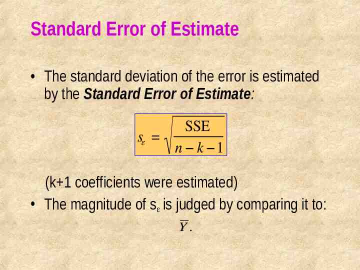
Standard Error of Estimate The standard deviation of the error is estimated by the Standard Error of Estimate: SSE sε n k 1 (k 1 coefficients were estimated) The magnitude of s is judged by comparing it to: Y.
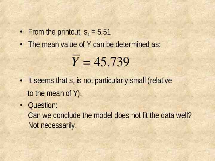
From the printout, s 5.51 The mean value of Y can be determined as: Y 45.739 It seems that s is not particularly small (relative to the mean of Y). Question: Can we conclude the model does not fit the data well? Not necessarily.
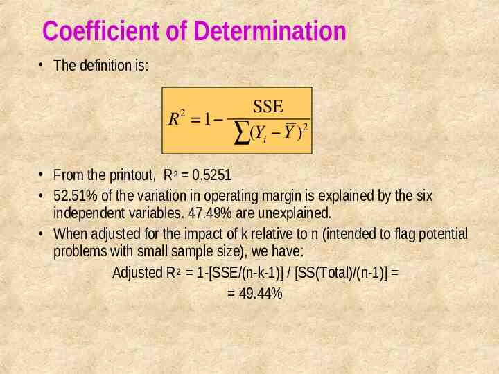
Coefficient of Determination The definition is: SSE R 1 2 (Y Y ) i 2 From the printout, R2 0.5251 52.51% of the variation in operating margin is explained by the six independent variables. 47.49% are unexplained. When adjusted for the impact of k relative to n (intended to flag potential problems with small sample size), we have: Adjusted R2 1-[SSE/(n-k-1)] / [SS(Total)/(n-1)] 49.44%
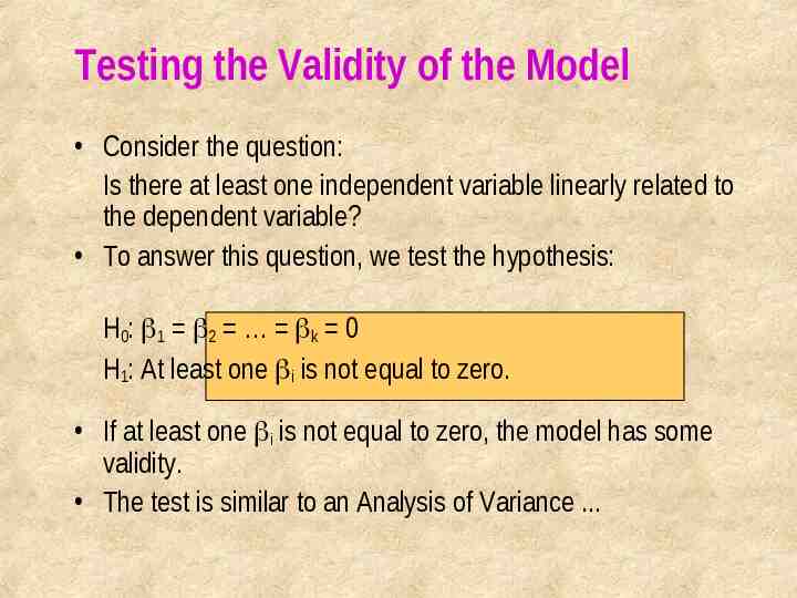
Testing the Validity of the Model Consider the question: Is there at least one independent variable linearly related to the dependent variable? To answer this question, we test the hypothesis: H0: 1 2 k 0 H1: At least one i is not equal to zero. If at least one i is not equal to zero, the model has some validity. The test is similar to an Analysis of Variance .
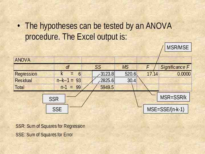
The hypotheses can be tested by an ANOVA procedure. The Excel output is: MSR/MSE ANOVA df Regression Residual Total k 6 n–k–1 93 n-1 99 SSR SSE SSR: Sum of Squares for Regression SSE: Sum of Squares for Error SS 3123.8 2825.6 5949.5 MS 520.6 30.4 F Significance F 17.14 0.0000 MSR SSR/k MSE SSE/(n-k-1)
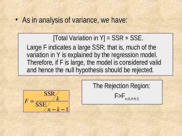
As in analysis of variance, we have: [Total Variation in Y] SSR SSE. Large F indicates a large SSR; that is, much of the variation in Y is explained by the regression model. Therefore, if F is large, the model is considered valid and hence the null hypothesis should be rejected. SSR F SSE k n k 1 The Rejection Region: F F ,k,n-k-1
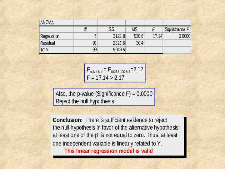
ANOVA df Regression Residual Total 6 93 99 SS 3123.8 2825.6 5949.5 MS 520.6 30.4 F Significance F 17.14 0.0000 F ,k,n-k-1 F0.05,6,100-6-1 2.17 F 17.14 2.17 Also, the p-value (Significance F) 0.0000 Reject the null hypothesis. Conclusion: Conclusion: There Thereisissufficient sufficientevidence evidencetotoreject reject the thenull nullhypothesis hypothesisininfavor favorofofthe thealternative alternativehypothesis: hypothesis: atatleast not equal to zero. Thus, at least leastone oneofofthe the i is i is not equal to zero. Thus, at least one oneindependent independentvariable variableisislinearly linearlyrelated relatedtotoY.Y. This Thislinear linearregression regressionmodel modelisisvalid valid
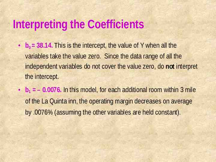
Interpreting the Coefficients b0 38.14. This is the intercept, the value of Y when all the variables take the value zero. Since the data range of all the independent variables do not cover the value zero, do not interpret the intercept. b1 – 0.0076. In this model, for each additional room within 3 mile of the La Quinta inn, the operating margin decreases on average by .0076% (assuming the other variables are held constant).
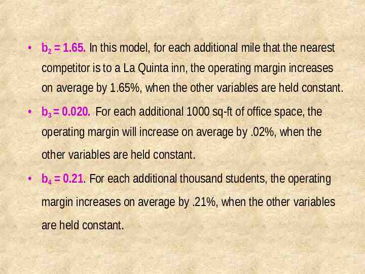
b2 1.65. In this model, for each additional mile that the nearest competitor is to a La Quinta inn, the operating margin increases on average by 1.65%, when the other variables are held constant. b3 0.020. For each additional 1000 sq-ft of office space, the operating margin will increase on average by .02%, when the other variables are held constant. b4 0.21. For each additional thousand students, the operating margin increases on average by .21%, when the other variables are held constant.
b5 0.41. For each increment of 1000 in median household income, the operating margin would increase on average by .41%, when the other variables remain constant. b6 -0.23. For each additional mile to the downtown center, the operating margin decreases on average by .23%, when the other variables are held constant.
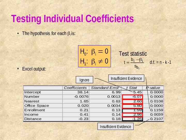
Testing Individual Coefficients The hypothesis for each i is: Excel output: H0: i 0 H1: i 0 Ignore Intercept Number Nearest Office Space Enrollment Income Distance Test statistic b βi t i sbi d.f. n - k -1 Insufficient Evidence Coefficients Standard Error 38.14 6.99 -0.0076 0.0013 1.65 0.63 0.020 0.0034 0.21 0.13 0.41 0.14 -0.23 0.18 t Stat 5.45 -6.07 2.60 5.80 1.59 2.96 -1.26 Insufficient Evidence P-value 0.0000 0.0000 0.0108 0.0000 0.1159 0.0039 0.2107
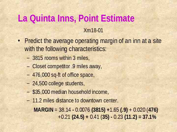
La Quinta Inns, Point Estimate Xm18-01 Predict the average operating margin of an inn at a site with the following characteristics: – – – – – – 3815 rooms within 3 miles, Closet competitor .9 miles away, 476,000 sq-ft of office space, 24,500 college students, 35,000 median household income, 11.2 miles distance to downtown center. MARGIN 38.14 - 0.0076 (3815) 1.65 (.9) 0.020 (476) 0.21 (24.5) 0.41 (35) - 0.23 (11.2) 37.1%
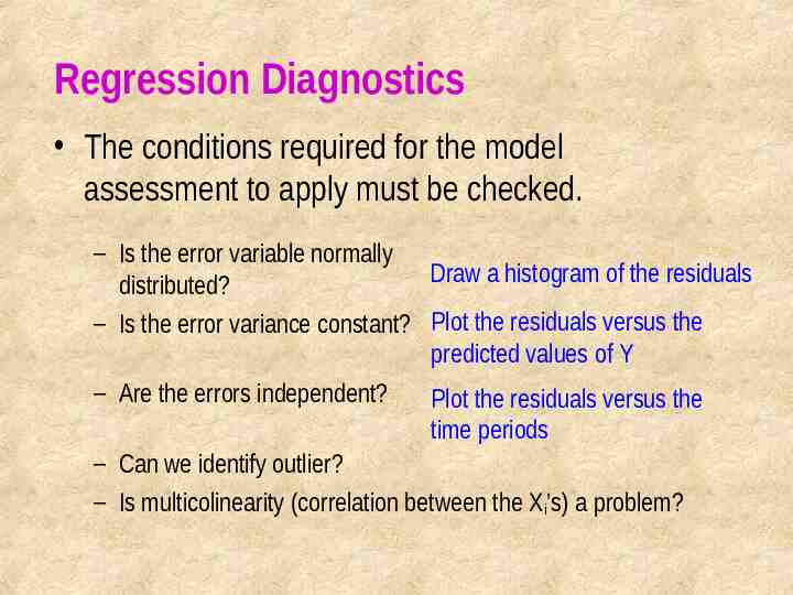
Regression Diagnostics The conditions required for the model assessment to apply must be checked. – Is the error variable normally Draw a histogram of the residuals distributed? – Is the error variance constant? Plot the residuals versus the predicted values of Y – Are the errors independent? Plot the residuals versus the time periods – Can we identify outlier? – Is multicolinearity (correlation between the Xi’s) a problem?