Standard Options: Call Definition A standard call is an option

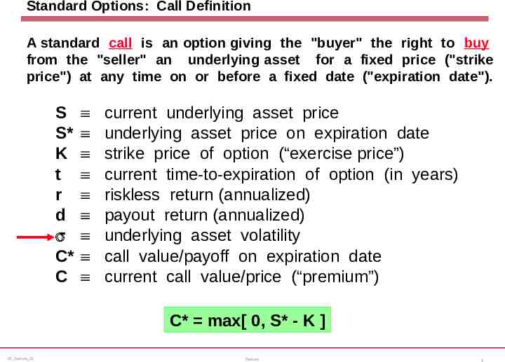
Standard Options: Call Definition A standard call is an option giving the "buyer" the right to buy from the "seller" an "underlying asset" for a fixed price ("strike price") at any time on or before a fixed date ("expiration date"). S S* K t r d s C* C º º º º º º º º º current underlying asset price underlying asset price on expiration date strike price of option (“exercise price”) current time-to-expiration of option (in years) riskless return (annualized) payout return (annualized) underlying asset volatility call value/payoff on expiration date current call value/price (“premium”) C* C* max[ max[0, 0, S* S* -- KK]] CF Options 21 Options 1

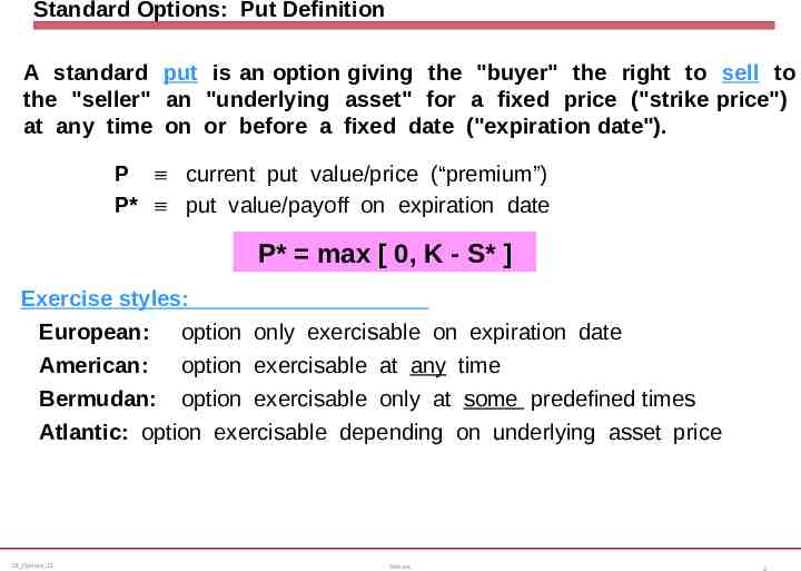
Standard Options: Put Definition A standard put is an option giving the "buyer" the right to sell to the "seller" an "underlying asset" for a fixed price ("strike price") at any time on or before a fixed date ("expiration date"). P º current put value/price (“premium”) P* º put value/payoff on expiration date P* P* max max [[0, 0, KK-- S* S*]] Exercise styles: European: option only exercisable on expiration date American: option exercisable at any time Bermudan: option exercisable only at some predefined times Atlantic: option exercisable depending on underlying asset price CF Options 21 Options 2

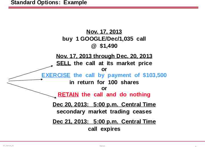
Standard Options: Example Nov. 17, 2013 buy 1 GOOGLE/Dec/1,035 call @ 1,490 Nov. 17, 2013 through Dec. 20, 2013 SELL the call at its market price or EXERCISE the call by payment of 103,500 in return for 100 shares or RETAIN the call and do nothing Dec 20, 2013: 5:00 p.m. Central Time secondary market trading ceases Dec 21, 2013: 5:00 p.m. Central Time call expires CF Options 21 Options 3

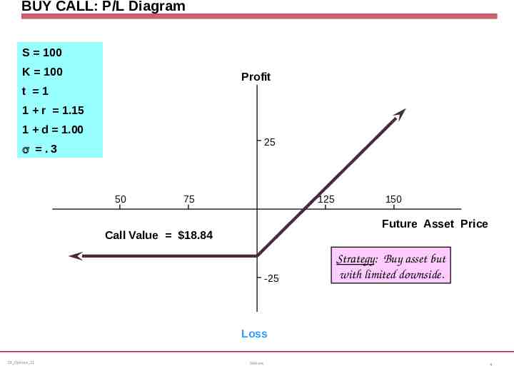
BUY CALL: P/L Diagram S 100 K 100 Profit t 1 1 r 1.15 1 d 1.00 25 s .3 50 75 125 150 Future Asset Price Call Value 18.84 -25 Strategy: Strategy: Buy Buyasset assetbut but with withlimited limiteddownside. downside. Loss CF Options 21 Options 4

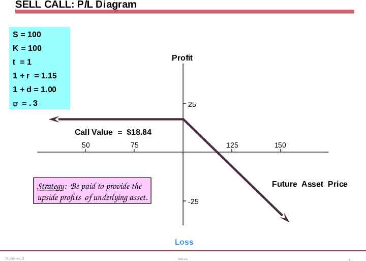
SELL CALL: P/L Diagram S 100 K 100 Profit t 1 1 r 1.15 1 d 1.00 s .3 25 Call Value 18.84 50 75 125 150 Future Asset Price Strategy: Strategy: Be Bepaid paidtotoprovide providethe the upside upsideprofits profits ofofunderlying underlyingasset. asset. -25 Loss CF Options 21 Options 5

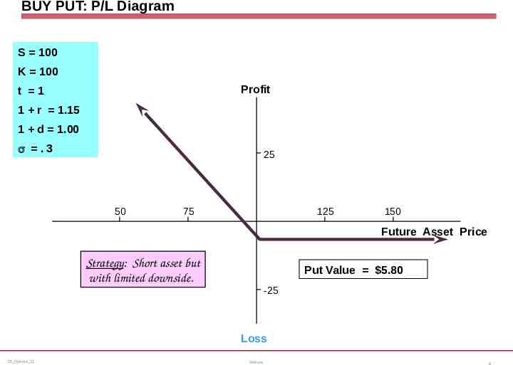
BUY PUT: P/L Diagram S 100 K 100 Profit t 1 1 r 1.15 1 d 1.00 s .3 25 50 75 125 150 Future Asset Price Strategy: Strategy: Short Shortasset assetbut but with withlimited limiteddownside. downside. Put Value 5.80 -25 Loss CF Options 21 Options 6

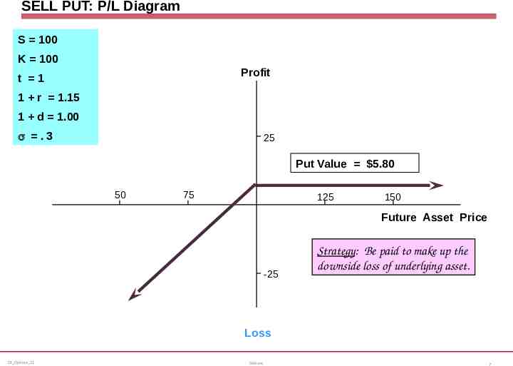
SELL PUT: P/L Diagram S 100 K 100 Profit t 1 1 r 1.15 1 d 1.00 s .3 25 Put Value 5.80 50 75 125 150 Future Asset Price -25 Strategy: Strategy: Be Bepaid paidtotomake makeup upthe the downside downsideloss lossofofunderlying underlyingasset. asset. Loss CF Options 21 Options 7

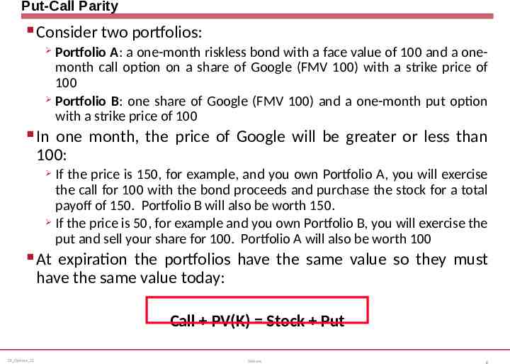
Put-Call Parity Consider two portfolios: Portfolio A: a one-month riskless bond with a face value of 100 and a onemonth call option on a share of Google (FMV 100) with a strike price of 100 Portfolio B: one share of Google (FMV 100) and a one-month put option with a strike price of 100 In one month, the price of Google will be greater or less than 100: If the price is 150, for example, and you own Portfolio A, you will exercise the call for 100 with the bond proceeds and purchase the stock for a total payoff of 150. Portfolio B will also be worth 150. If the price is 50, for example and you own Portfolio B, you will exercise the put and sell your share for 100. Portfolio A will also be worth 100 At expiration the portfolios have the same value so they must have the same value today: Call PV(K) Stock Put CF Options 21 Options 8

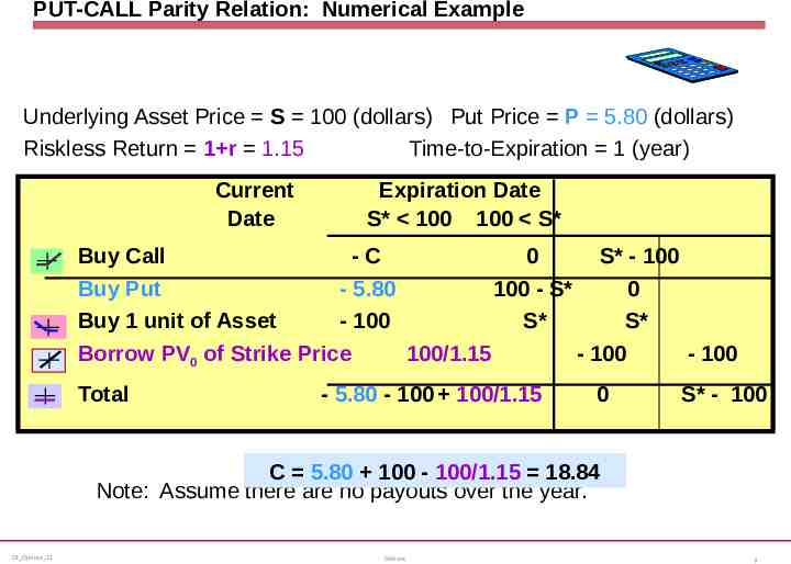
PUT-CALL Parity Relation: Numerical Example Underlying Asset Price S 100 (dollars) Put Price P 5.80 (dollars) Riskless Return 1 r 1.15 Time-to-Expiration 1 (year) Current Date Expiration Date S* 100 100 S* Buy Call -C 0 S* - 100 Buy Put - 5.80 100 - S* 0 Buy 1 unit of Asset - 100 S* S* Borrow PV0 of Strike Price 100/1.15 - 100 - 100 Total - 5.80 - 100 100/1.15 0 S* - 100 C 5.80 100 - 100/1.15 18.84 Note: Assume there are no payouts over the year. CF Options 21 Options 9

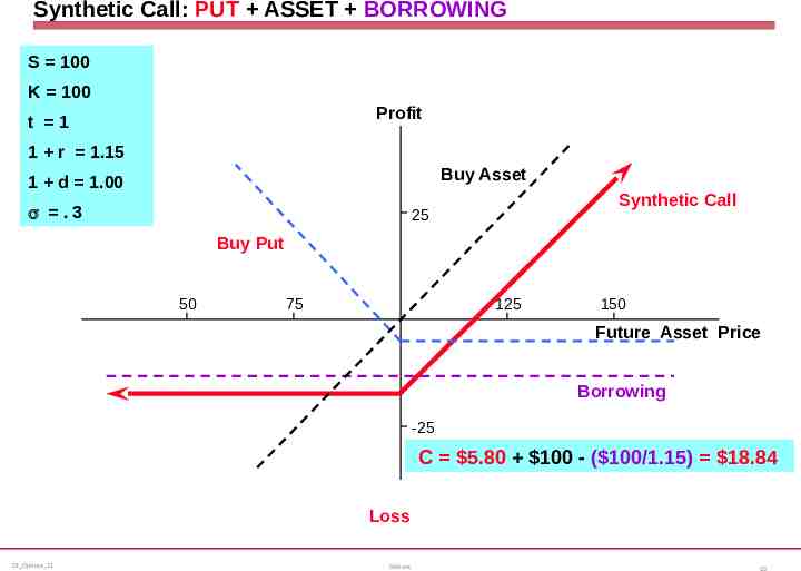
Synthetic Call: PUT ASSET BORROWING S 100 K 100 Profit t 1 1 r 1.15 Buy Asset 1 d 1.00 s .3 Synthetic Call 25 Buy Put 50 75 125 150 Future Asset Price Borrowing -25 C 5.80 100 - ( 100/1.15) 18.84 Loss CF Options 21 Options 10

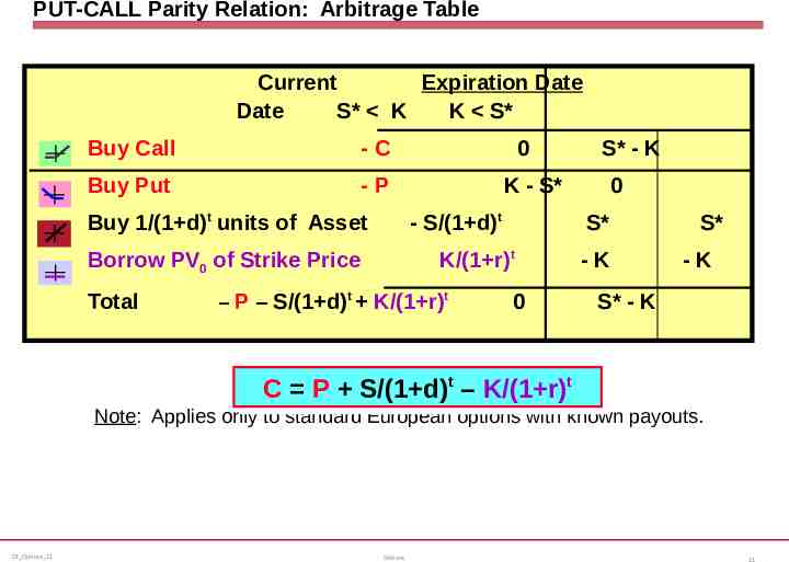
PUT-CALL Parity Relation: Arbitrage Table Current Expiration Date Date S* K K S* Buy Call -C Buy Put -P Buy 1/(1 d)t units of Asset S* - K K - S* - S/(1 d)t – P – S/(1 d)t K/(1 r)t 0 S* K/(1 r)t Borrow PV0 of Strike Price Total 0 0 -K S* -K S* - K tt tt CC PP S/(1 d) – K/(1 r) S/(1 d) – K/(1 r) Note: Applies only to standard European options with known payouts. CF Options 21 Options 11

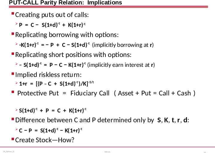
PUT-CALL Parity Relation: Implications Creating puts out of calls: P C – S(1 d)-t K(1 r)-t Replicating borrowing with options: -K(1 r)-t – P C – S(1 d)-t (implicitly borrowing at r) Replicating short positions with options: – S(1 d)-t P – C – K(1 r)-t (implicitly earn interest at r) Implied riskless return: 1 r [(P – C S(1 d)-t )/K]-1/t Protective Put Fiduciary Call ( Asset Put Call Cash ) S(1 d)-t P C K(1 r)-t Difference between C and P determined only by S, K, t, r, d: C – P S(1 d)-t – K(1 r)-t Create Stock—How? CF Options 21 Options 12

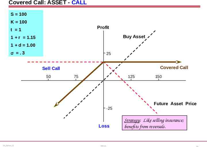
Covered Call: ASSET - CALL S 100 K 100 Profit t 1 Buy Asset 1 r 1.15 1 d 1.00 s .3 25 Covered Call Sell Call 50 75 125 -25 Loss CF Options 21 Options 150 Future Asset Price Strategy: Strategy: Like Likeselling sellinginsurance; insurance; benefits from reversals. benefits from reversals. 13

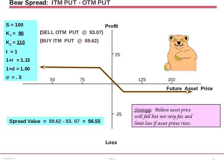
Bear Spread: ITM PUT - OTM PUT S 100 Profit K1 90 (SELL OTM PUT @ 3.07) K2 110 (BUY ITM PUT @ 9.62) t 1 25 1 r 1.15 1 d 1.00 s .3 50 75 125 150 Future Asset Price -25 Spread Value 9.62 - 3. 07 6.55 Strategy: Strategy: Believe Believeasset assetprice price will willfall fallbut butnot notvery veryfar, far,and and limit limitloss lossififasset assetprices pricesrises. rises. Loss CF Options 21 Options 14

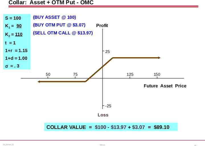
Collar: Asset OTM Put - OMC S 100 (BUY ASSET @ 100) K1 90 (BUY OTM PUT @ 3.07) K2 110 (SELL OTM CALL @ 13.97) Profit t 1 1 r 1.15 25 1 d 1.00 s .3 50 75 125 150 Future Asset Price -25 Loss COLLAR VALUE 100 - 13.97 3.07 89.10 CF Options 21 Options 15

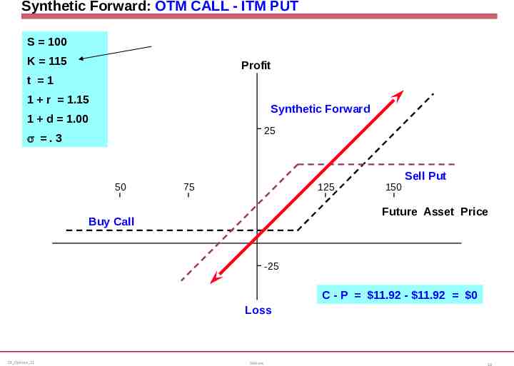
Synthetic Forward: OTM CALL - ITM PUT S 100 K 115 Profit t 1 1 r 1.15 Synthetic Forward 1 d 1.00 25 s .3 50 75 125 150 Sell Put Future Asset Price Buy Call -25 C - P 11.92 - 11.92 0 Loss CF Options 21 Options 16

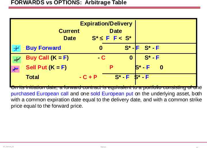
FORWARDS vs OPTIONS: Arbitrage Table Expiration/Delivery Current Date Date S* F F S* Buy Forward 0 Buy Call (K F) -C Sell Put (K F) Total S* - F S* - F 0 P -C P S* - F S* - F 0 S* - F S* - F On its initiation date, a forward contract is equivalent to a portfolio consisting of one purchased European call and one sold European put on the underlying asset, both with a common expiration date equal to the delivery date, and with a common strike price equal to the forward price. CF Options 21 Options 17

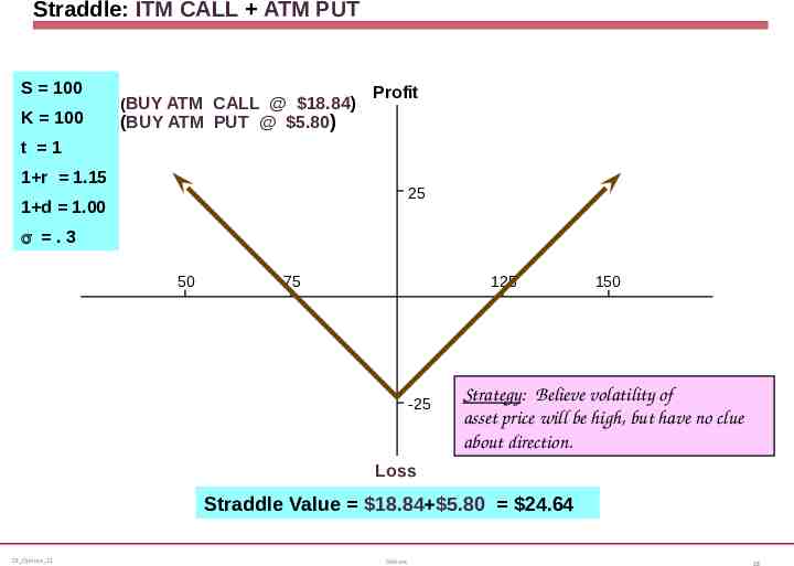
Straddle: ITM CALL ATM PUT S 100 K 100 (BUY ATM CALL @ 18.84) Profit (BUY ATM PUT @ 5.80) t 1 1 r 1.15 25 1 d 1.00 s .3 50 75 125 -25 Loss 150 Strategy: ofof Future Price Strategy: Believe Believevolatility volatilityAsset asset assetprice pricewill willbebehigh, high,but buthave haveno noclue clue about aboutdirection. direction. Straddle Value 18.84 5.80 24.64 CF Options 21 Options 18

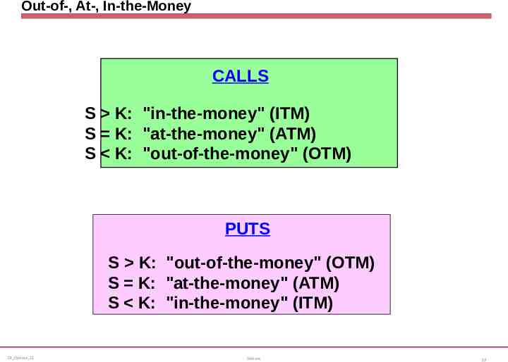
Out-of-, At-, In-the-Money CALLS S K: "in-the-money" (ITM) S K: "at-the-money" (ATM) S K: "out-of-the-money" (OTM) PUTS S K: "out-of-the-money" (OTM) S K: "at-the-money" (ATM) S K: "in-the-money" (ITM) CF Options 21 Options 19

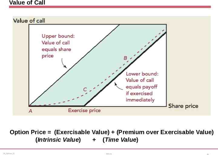
Value of Call Option Price (Exercisable Value) (Premium over Exercisable Value) (Intrinsic Value) (Time Value) CF Options 21 Options 20

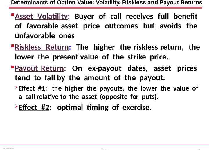
Determinants of Option Value: Volatility, Riskless and Payout Returns Asset Volatility: Buyer of call receives full benefit of favorable asset price outcomes but avoids the unfavorable ones Riskless Return: The higher the riskless return, the lower the present value of the strike price. Payout Return: On ex-payout dates, asset prices tend to fall by the amount of the payout. CF Options 21 Effect #1: the higher the payouts, the lower the value of a call relative to the asset (opposite for puts). Effect #2: optimal timing of exercise. Options 21

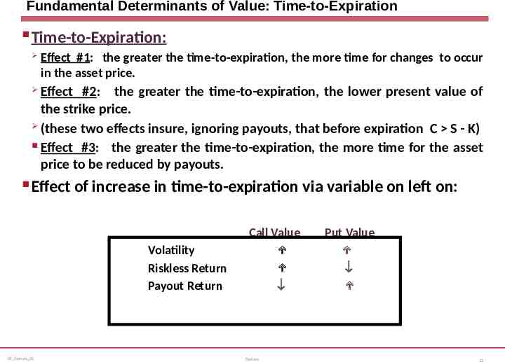
Fundamental Determinants of Value: Time-to-Expiration Time-to-Expiration: Effect #1: the greater the time-to-expiration, the more time for changes to occur in the asset price. Effect #2: the greater the time-to-expiration, the lower present value of the strike price. (these two effects insure, ignoring payouts, that before expiration C S - K) Effect #3: the greater the time-to-expiration, the more time for the asset price to be reduced by payouts. Effect of increase in time-to-expiration via variable on left on: Volatility Riskless Return Payout Return CF Options 21 Call Value Options Put Value 22

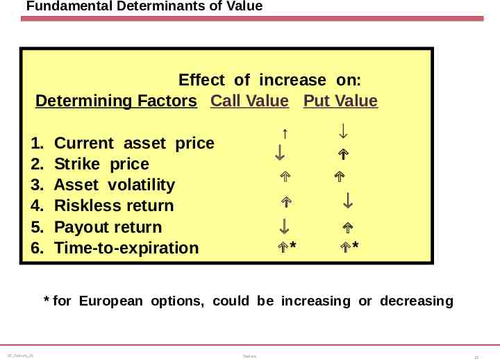
Fundamental Determinants of Value Effect of increase on: Determining Factors Call Value Put Value 1. 2. 3. 4. 5. 6. Current asset price Strike price Asset volatility Riskless return Payout return Time-to-expiration * * * for European options, could be increasing or decreasing CF Options 21 Options 23

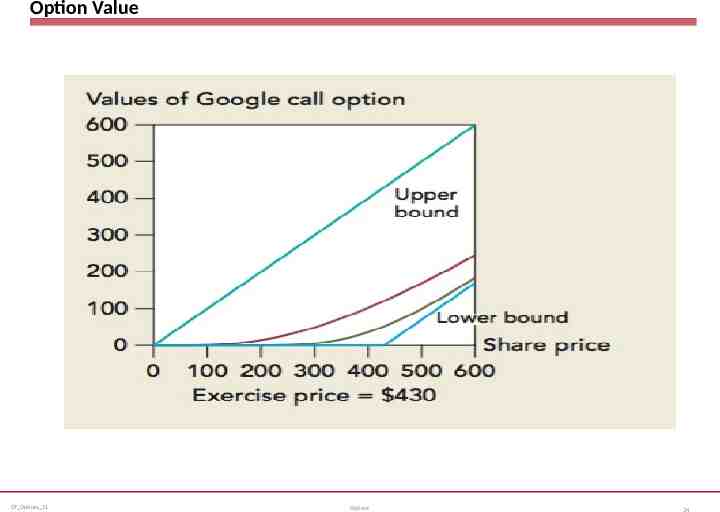
Option Value CF Options 21 Options 24

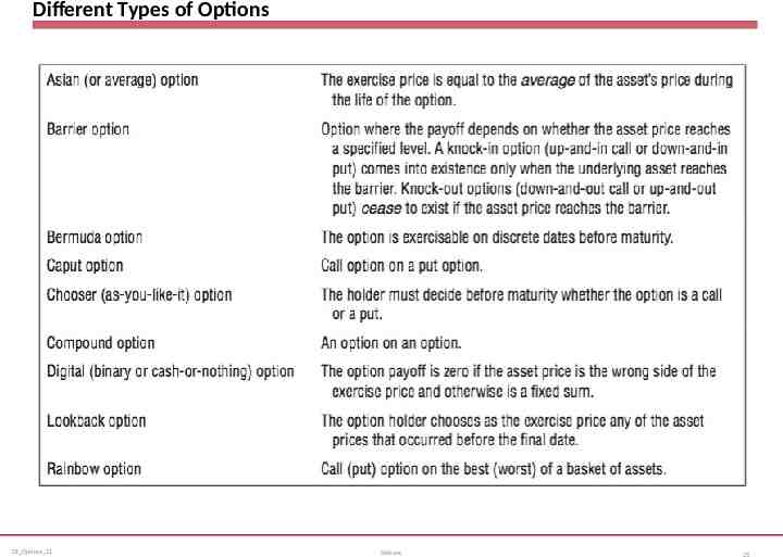
Different Types of Options CF Options 21 Options 25

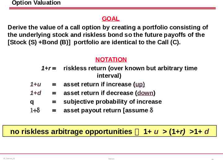
Option Valuation GOAL Derive the value of a call option by creating a portfolio consisting of the underlying stock and riskless bond so the future payoffs of the [Stock (S) Bond (B)] portfolio are identical to the Call (C). 1 r º 1 u 1 d q 1 d º º º º NOTATION riskless return (over known but arbitrary time interval) asset return if increase (up) asset return if decrease (down) subjective probability of increase asset payout return [assume d no riskless arbitrage opportunities 1 u (1 r) 1 d CF Options 21 Options 26

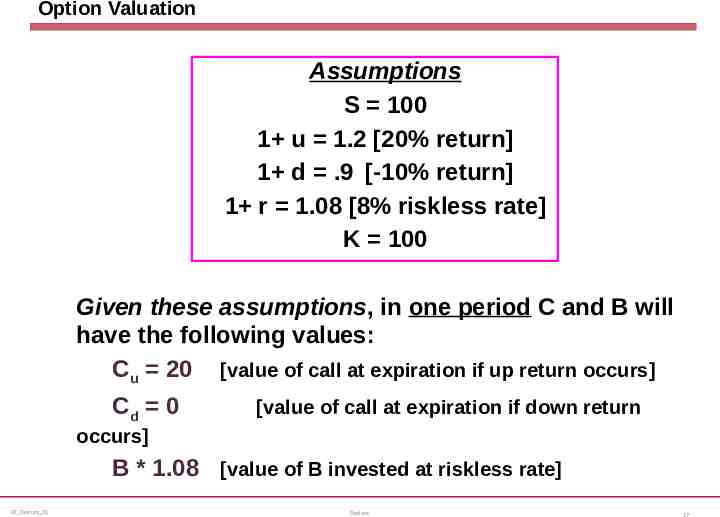
Option Valuation Assumptions S 100 1 u 1.2 [20% return] 1 d .9 [-10% return] 1 r 1.08 [8% riskless rate] K 100 Given these assumptions, in one period C and B will have the following values: Cu 20 [value of call at expiration if up return occurs] Cd 0 [value of call at expiration if down return occurs] B * 1.08 [value of B invested at riskless rate] CF Options 21 Options 27

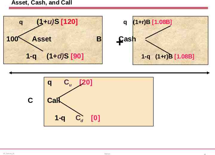
Asset, Cash, and Call (1 u)S [120] q 100 Asset 1-q C Cash (1 d)S [90] Cu (1 r)B [1.08B] B q 1-q (1 r)B [1.08B] [20] Call 1-q CF Options 21 q Cd [0] Options 28

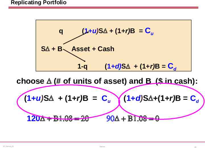
Replicating Portfolio q SD B (1 u)SD (1 r)B Cu Asset Cash 1-q (1 d)SD (1 r)B Cd choose D (# of units of asset) and B ( in cash): (1 u)SD (1 r)B Cu 120D B1.08 20 CF Options 21 (1 d)SD (1 r)B Cd 90D B1.08 0 Options 29

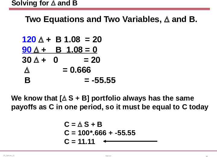
Solving for D and B Two Equations and Two Variables, D and B. 120 D B 1.08 20 90 D B 1.08 0 30 D 0 20 D 0.666 B -55.55 We know that [D S B] portfolio always has the same payoffs as C in one period, so it must be equal to C today C DS B C 100*.666 -55.55 C 11.11 CF Options 21 Options 30

General Formulas for D and B CF Options 21 Options 31

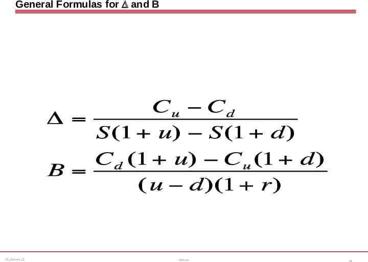
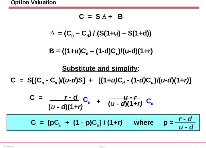
Option Valuation C SD B D (Cu – Cd) / (S(1 u) – S(1 d)) B ((1 u)Cd – (1-d)Cu)/(u-d)(1 r) Substitute and simplify: C S[(Cu - Cd )/(u-d)S] [(1 u)Cd - (1-d)Cu )/(u-d)(1 r)] C r-d C u (u - d)(1 r) u-r (u - d)(1 r) Cd CC [pC [pCuu (1 (1-- p)C p)Cdd]] //(1 r) (1 r) CF Options 21 Options where where r-d pp u-d 32

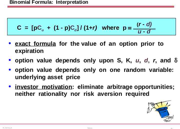
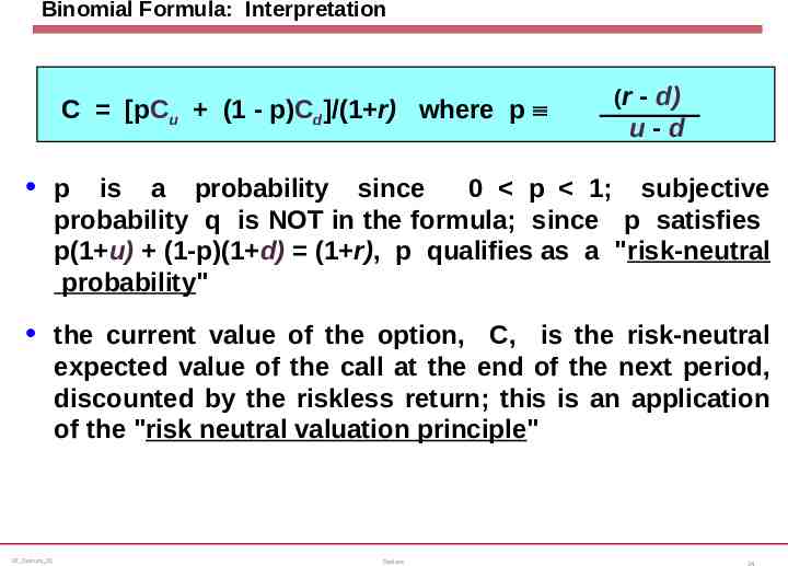
Binomial Formula: Interpretation C [pCu (1 - p)Cd] / (1 r) where p º (r - d) u-d exact formula for the value of an option prior to expiration option value depends only upon S, K, u, d, r, and d option value depends only on one random variable: underlying asset price investor motivation: eliminate arbitrage opportunities; neither rationality nor risk aversion required CF Options 21 Options 33

Binomial Formula: Interpretation C [pCu (1 - p)Cd]/(1 r) where p º (r - d) u-d p is a probability since 0 p 1; subjective probability q is NOT in the formula; since p satisfies p(1 u) (1-p)(1 d) (1 r), p qualifies as a "risk-neutral probability" the current value of the option, C, is the risk-neutral expected value of the call at the end of the next period, discounted by the riskless return; this is an application of the "risk neutral valuation principle" CF Options 21 Options 34

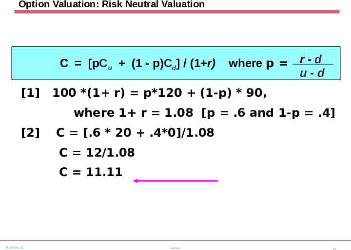
Option Valuation: Risk Neutral Valuation r-d CC [pC [pCuu (1 (1 --p)C p)Cdd]] // (1 r) (1 r) where where pp u-d [1] 100 *(1 r) p*120 (1-p) * 90, where 1 r 1.08 [p .6 and 1-p .4] [2] C [.6 * 20 .4*0]/1.08 C 12/1.08 C 11.11 CF Options 21 Options 35

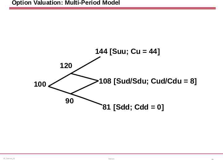
Option Valuation: Multi-Period Model 144 [Suu; Cu 44] 120 108 [Sud/Sdu; Cud/Cdu 8] 100 90 CF Options 21 81 [Sdd; Cdd 0] Options 36

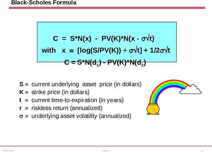
Black-Scholes Formula C S*N(x) - PV(K)*N(x - sÖt) with x º [log(S/PV(K)) sÖt] 1/2sÖt C S*N(d1) - PV(K)*N(d2) Sº Kº t º r º sº CF Options 21 current underlying asset price (in dollars) strike price (in dollars) current time-to-expiration (in years) riskless return (annualized) underlying asset volatility (annualized) Options 37

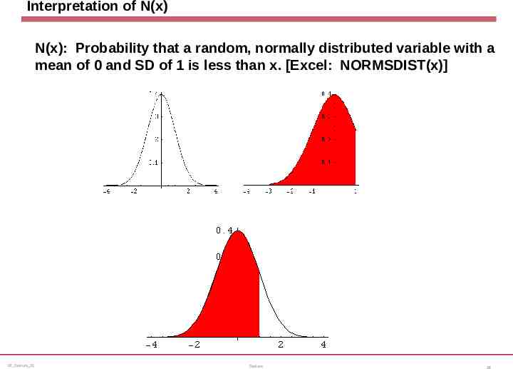
Interpretation of N(x) N(x): Probability that a random, normally distributed variable with a mean of 0 and SD of 1 is less than x. [Excel: NORMSDIST(x)] CF Options 21 Options 38

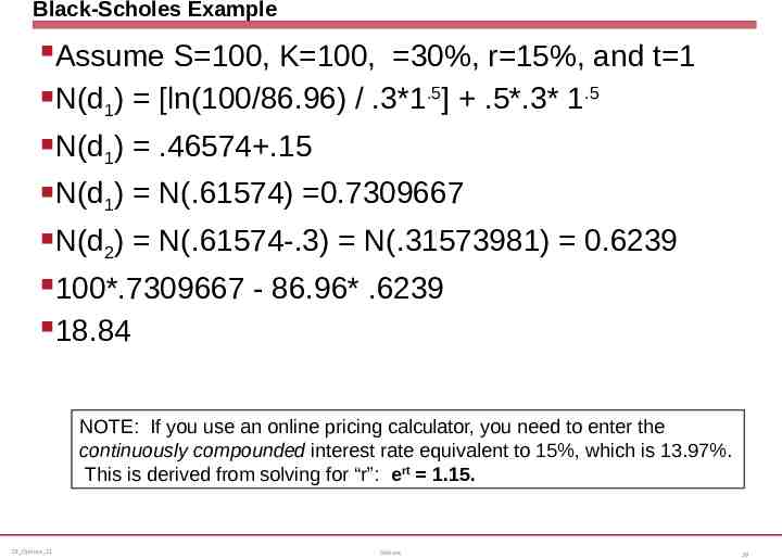
Black-Scholes Example Assume S 100, K 100, 30%, r 15%, and t 1 N(d ) [ln(100/86.96) / .3*1.5] .5*.3* 1.5 1 N(d1) .46574 .15 N(d1) N(.61574) 0.7309667 N(d2) N(.61574-.3) N(.31573981) 0.6239 100*.7309667 - 86.96* .6239 18.84 NOTE: If you use an online pricing calculator, you need to enter the continuously compounded interest rate equivalent to 15%, which is 13.97%. This is derived from solving for “r”: ert 1.15. CF Options 21 Options 39

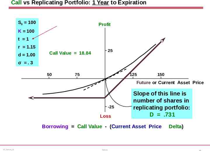
Call vs Replicating Portfolio: 1 Year to Expiration S0 100 Profit K 100 t 1 r 1.15 d 1.00 25 Call Value 18.84 σ .3 50 75 125 150 Future or Current Asset Price -25 Loss Slope Slopeof ofthis thisline lineis is number numberof ofshares sharesin in replicating replicatingportfolio: portfolio: DD .731 .731 Borrowing Call Value - (Current Asset Price Delta) CF Options 21 Options 40

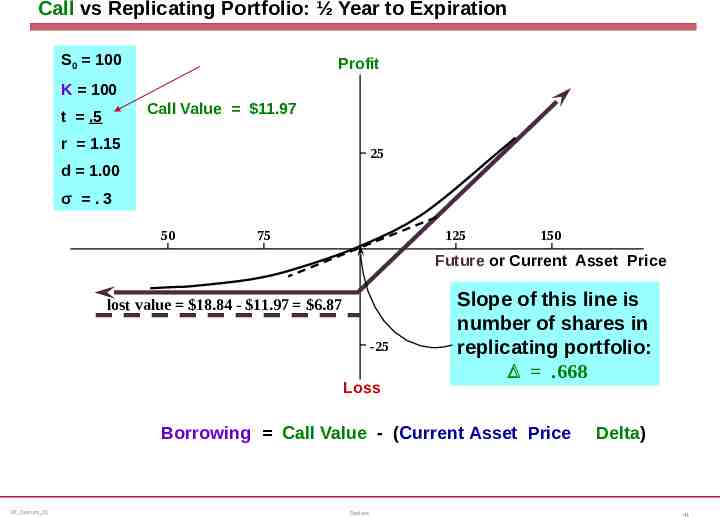
Call vs Replicating Portfolio: ½ Year to Expiration S0 100 Profit K 100 Call Value 11.97 t .5 r 1.15 25 d 1.00 σ .3 50 75 125 150 Future or Current Asset Price lost value 18.84 - 11.97 6.87 -25 Loss Slope Slopeof ofthis thisline lineis is number numberof ofshares sharesin in replicating replicatingportfolio: portfolio: DD .668 .668 Borrowing Call Value - (Current Asset Price Delta) CF Options 21 Options 41

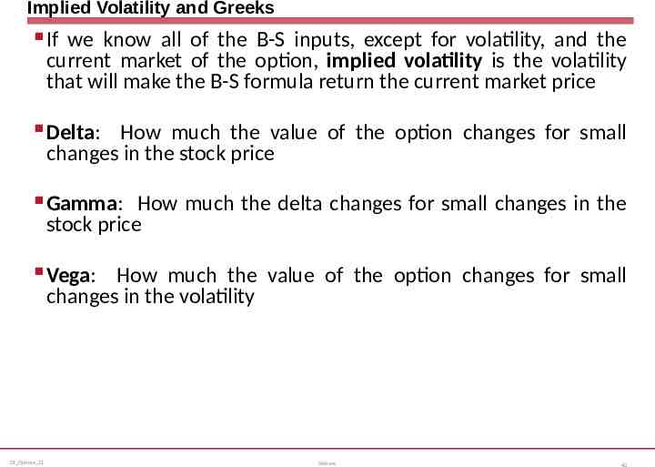
Implied Volatility and Greeks If we know all of the B-S inputs, except for volatility, and the current market of the option, implied volatility is the volatility that will make the B-S formula return the current market price Delta: How much the value of the option changes for small changes in the stock price Gamma: How much the delta changes for small changes in the stock price Vega: How much the value of the option changes for small changes in the volatility CF Options 21 Options 42

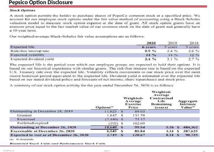
Pepsico Option Disclosure CF Options 21 Options 43

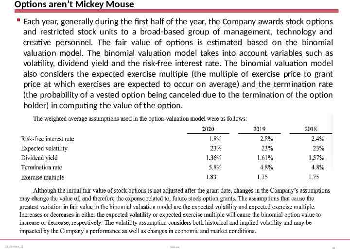
Options aren’t Mickey Mouse Each year, generally during the first half of the year, the Company awards stock options and restricted stock units to a broad-based group of management, technology and creative personnel. The fair value of options is estimated based on the binomial valuation model. The binomial valuation model takes into account variables such as volatility, dividend yield and the risk-free interest rate. The binomial valuation model also considers the expected exercise multiple (the multiple of exercise price to grant price at which exercises are expected to occur on average) and the termination rate (the probability of a vested option being canceled due to the termination of the option holder) in computing the value of the option. CF Options 21 Options 44

The Firm as a Portfolio of Call Options For a company with debt: Shareholders can be viewed as having purchased a Call from the bondholders (strike face value of debt) If the value of the firm is greater than the debt, the SHs exercise the call and purchase the firm from the bondholders (pay back the debt). BHs can be seen as owning the firm and having sold a call option to SHs CF Options 21 Options 45

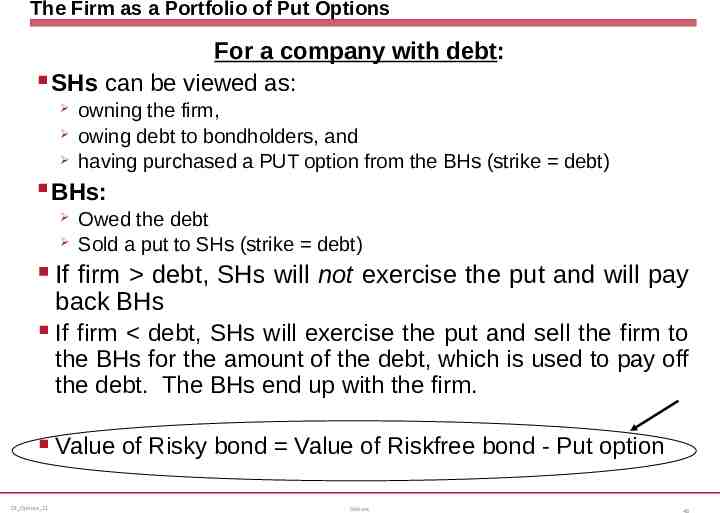
The Firm as a Portfolio of Put Options For a company with debt: SHs can be viewed as: owning the firm, owing debt to bondholders, and having purchased a PUT option from the BHs (strike debt) BHs: Owed the debt Sold a put to SHs (strike debt) If firm debt, SHs will not exercise the put and will pay back BHs If firm debt, SHs will exercise the put and sell the firm to the BHs for the amount of the debt, which is used to pay off the debt. The BHs end up with the firm. Value of Risky bond Value of Riskfree bond - Put option CF Options 21 Options 46

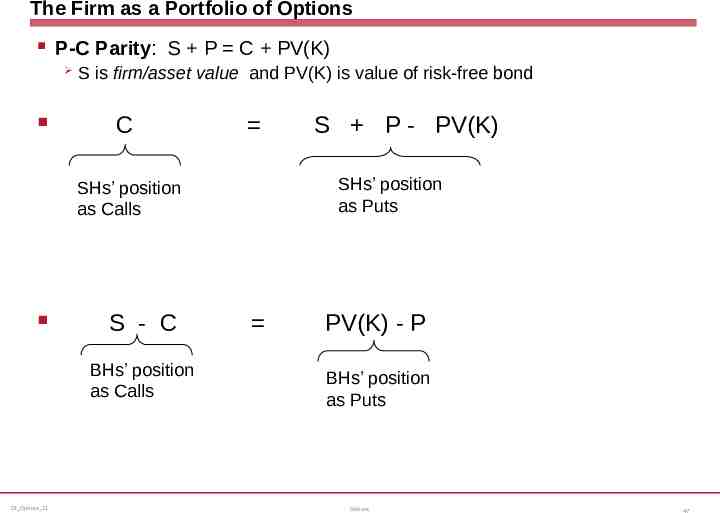
The Firm as a Portfolio of Options P-C Parity: S P C PV(K) S is firm/asset value and PV(K) is value of risk-free bond C SHs’ position as Puts SHs’ position as Calls S - C BHs’ position as Calls CF Options 21 S P - PV(K) PV(K) - P BHs’ position as Puts Options 47