Using Sector Valuations to Forecast Market Returns A Contrarian


16 Slides159.00 KB
Using Sector Valuations to Forecast Market Returns A Contrarian View February 27, 2003 Lewis Kaufman, CFA Cira Qin Justin Robert Shannon Thomas Vidhi Tambiah 1
Table of Contents Overview Using Sector Valuations to Forecast Market Returns Methodology A Contrarian View Regression Results Out-of-Sample Limited Data, Promising Results Trading Strategy ARCH The Model’s Predictive Power A Long-Short Approach Using Conditional Variance Conclusions 2
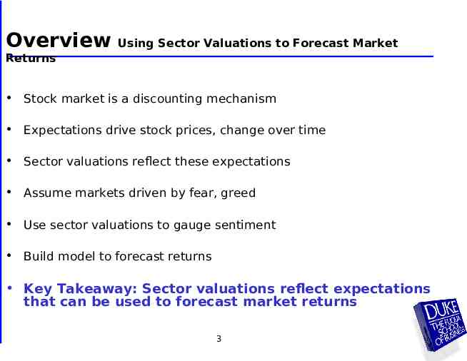
Overview Using Sector Valuations to Forecast Market Returns Stock market is a discounting mechanism Expectations drive stock prices, change over time Sector valuations reflect these expectations Assume markets driven by fear, greed Use sector valuations to gauge sentiment Build model to forecast returns Key Takeaway: Sector valuations reflect expectations that can be used to forecast market returns 3
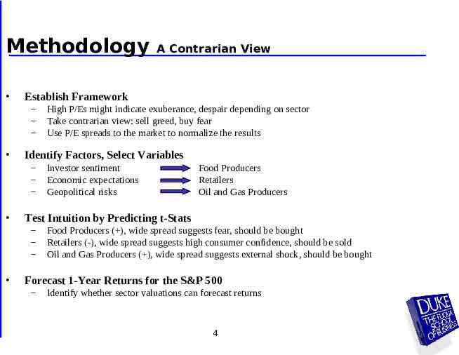
Methodology Establish Framework – – – Investor sentiment Economic expectations Geopolitical risks Food Producers Retailers Oil and Gas Producers Test Intuition by Predicting t-Stats – – – High P/Es might indicate exuberance, despair depending on sector Take contrarian view: sell greed, buy fear Use P/E spreads to the market to normalize the results Identify Factors, Select Variables – – – A Contrarian View Food Producers ( ), wide spread suggests fear, should be bought Retailers (-), wide spread suggests high consumer confidence, should be sold Oil and Gas Producers ( ), wide spread suggests external shock, should be bought Forecast 1-Year Returns for the S&P 500 – Identify whether sector valuations can forecast returns 4
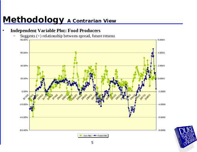
Methodology A Contrarian View Independent Variable Plot: Food Producers – Suggests ( ) relationship between spread, future returns 80.00% 6.0000 60.00% 4.0000 40.00% 2.0000 20.00% 0.0000 0.00% -2.0000 01 01 01 01 01 01 01 01 01 01 01 01 01 01 01 01 01 01 01 01 01 01 01 01 01 01 73 74 75 76 77 78 79 80 81 82 83 84 85 86 87 88 89 90 91 92 93 94 95 96 97 98 19 19 19 19 19 19 19 19 19 19 19 19 19 19 19 19 19 19 19 19 19 19 19 19 19 19 -20.00% -4.0000 -40.00% -6.0000 -60.00% -8.0000 Ann Ret 5 Food-Mkt
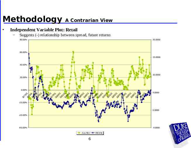
Methodology A Contrarian View Independent Variable Plot: Retail – Suggests (-) relationship between spread, future returns 80.00% 20.0000 60.00% 15.0000 40.00% 10.0000 20.00% 0.00% 01 01 01 01 01 01 01 01 01 01 01 01 01 01 01 01 01 01 01 01 01 01 01 01 01 01 73 974 975 976 977 978 979 980 981 982 983 984 985 986 987 988 989 990 991 992 993 994 995 996 997 998 9 1 1 1 1 1 1 1 1 1 1 1 1 1 1 1 1 1 1 1 1 1 1 1 1 1 1 5.0000 -20.00% 0.0000 -40.00% -60.00% -5.0000 Ann Ret 6 Rtl-Mkt
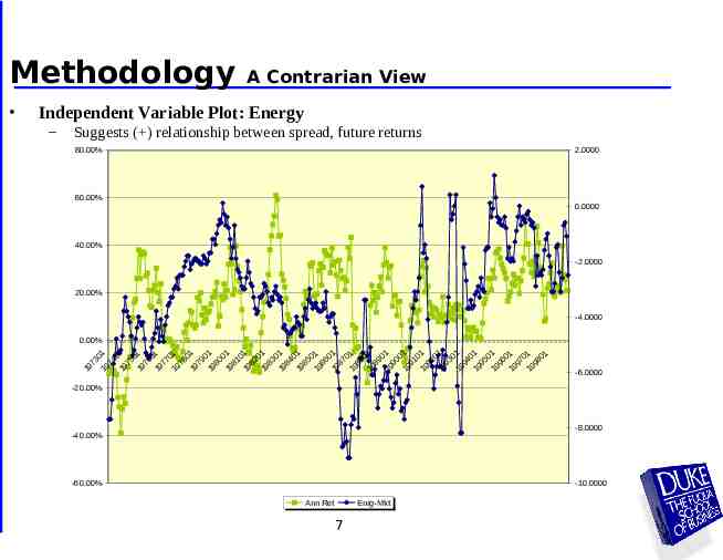
Methodology A Contrarian View Independent Variable Plot: Energy – Suggests ( ) relationship between spread, future returns 80.00% 2.0000 60.00% 0.0000 40.00% -2.0000 20.00% -4.0000 0.00% 01 01 01 01 01 01 01 01 01 01 01 01 01 01 01 01 01 01 01 01 01 01 01 01 01 01 73 974 975 976 977 978 979 980 981 982 983 984 985 986 987 988 989 990 991 992 993 994 995 996 997 998 9 1 1 1 1 1 1 1 1 1 1 1 1 1 1 1 1 1 1 1 1 1 1 1 1 1 1 -6.0000 -20.00% -8.0000 -40.00% -60.00% -10.0000 Ann Ret Enrg-Mkt 7
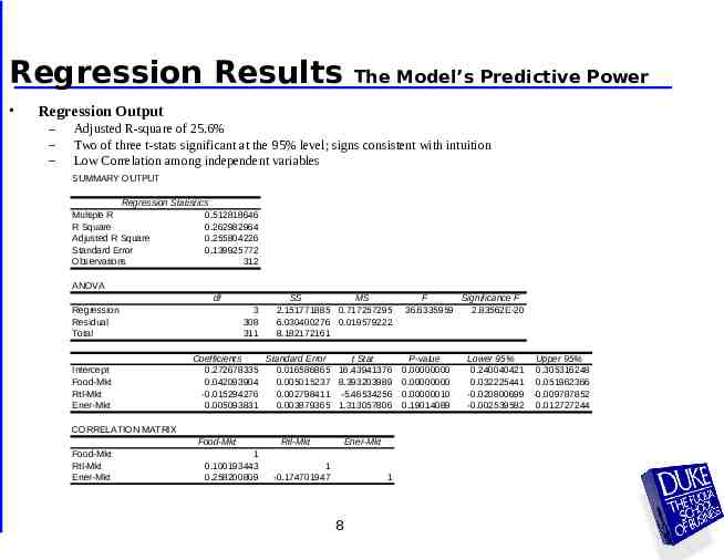
Regression Results The Model’s Predictive Power Regression Output – – – Adjusted R-square of 25.6% Two of three t-stats significant at the 95% level; signs consistent with intuition Low Correlation among independent variables SUMMARY OUTPUT Regression Statistics Multiple R 0.512818646 R Square 0.262982964 Adjusted R Square 0.255804226 Standard Error 0.139925772 Observations 312 ANOVA df Regression Residual Total Intercept Food-Mkt Rtl-Mkt Ener-Mkt 3 308 311 SS MS 2.151771885 0.717257295 6.030400276 0.019579222 8.182172161 Coefficients Standard Error t Stat 0.272678335 0.016586865 16.43941376 0.042093904 0.005015237 8.393203989 -0.015294276 0.002798411 -5.46534256 0.005093831 0.003879365 1.313057806 CORRELATION MATRIX Food-Mkt Food-Mkt Rtl-Mkt Ener-Mkt 1 0.100193443 0.258200809 Rtl-Mkt Ener-Mkt 1 -0.174701947 1 8 F Significance F 36.6335959 2.83562E-20 P-value 0.00000000 0.00000000 0.00000010 0.19014089 Lower 95% Upper 95% 0.240040421 0.305316248 0.032225441 0.051962366 -0.020800699 -0.009787852 -0.002539582 0.012727244
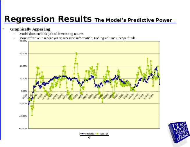
Regression Results The Model’s Predictive Power Graphically Appealing – – Model does credible job of forecasting returns More effective in recent years: access to information, trading volumes, hedge funds 80.00% 60.00% 40.00% 20.00% 0.00% 01 01 01 01 01 01 01 01 01 01 01 01 01 01 01 01 01 01 01 01 01 01 01 01 01 01 73 974 975 976 977 978 979 980 981 982 983 984 985 986 987 988 989 990 991 992 993 994 995 996 997 998 19 1 1 1 1 1 1 1 1 1 1 1 1 1 1 1 1 1 1 1 1 1 1 1 1 1 -20.00% -40.00% -60.00% Predicted 9 Ann Ret
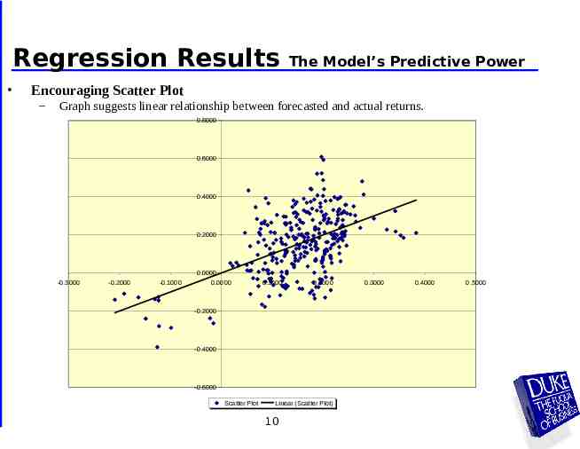
Regression Results The Model’s Predictive Power Encouraging Scatter Plot – Graph suggests linear relationship between forecasted and actual returns. 0.8000 0.6000 0.4000 0.2000 -0.3000 -0.2000 -0.1000 0.0000 0.0000 0.1000 0.2000 -0.2000 -0.4000 -0.6000 Scatter Plot Linear (Scatter Plot) 10 0.3000 0.4000 0.5000
Regression Results The Model’s Predictive Power Other Observations – – – – – Graph suggests linear relationship between forecasted and actual returns Systematic positive bias in-sample, results encouraging out-of-sample Strong predictor of directional change, implications for trading strategies Model more effective in recent years: access to information, hedge funds, volume Considered fitting in-sample data to more recent years and using an earlier period as out-of-sample. Better results for R-square and T-statistics. Dismissed idea because out-of-sample from past periods may not be indicative of success 11
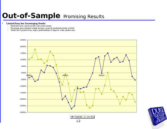
Out-of-Sample Promising Results Limited Data, but Encouraging Results – – – Predicted curve clearly trends with actual returns Promising given limited sample horizon; correctly predicted decline in 2000 Model has a positive bias, expect predictability to improve when market rises 25.00% 20.00% 15.00% 10.00% 5.00% 0.00% 199901 200001 200101 -5.00% -10.00% -15.00% -20.00% -25.00% -30.00% Predicted 12 Ann Ret
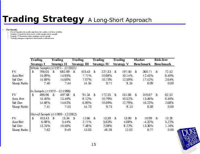
Trading Strategy A Long-Short Approach Basic Strategy: Long-Short Approach – – – – Invest 1 in 1/73, invest 1 in 2/73, invest 1 in 3/73, Reinvest proceeds from 1/73 on 1/74, reinvest 2/73 on 2/74, Long-Short investment decision based on model’s predictions Compare against benchmarks, market return and risk-free return Five Strategies – – – – Trading Strategy I: Trading Strategy II: Trading Strategy III: Trading Strategy IV: Conditional Variance – Trading Strategy V: Basic Long-Short Long-Short with Risk-free Long-Short with Momentum Conservative Long-Short with Long-Short with Conditional Variance 13
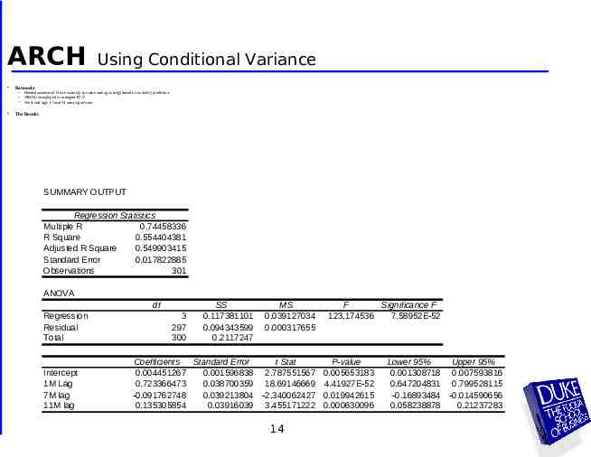
ARCH Rationale – – – Using Conditional Variance Needed measure of future volatility to create trading strategy based on volatility prediction ARCH is employed in strategies IV,V We found lags 1,7 and 11 most significant The Results SUMMARY OUTPUT Regression Statistics Multiple R 0.74458336 R Square 0.554404381 Adjusted R Square 0.549903415 Standard Error 0.017822885 Observations 301 ANOVA df Regression Residual Total Intercept 1M Lag 7M lag 11M lag 3 297 300 SS 0.117381101 0.094343599 0.2117247 MS 0.039127034 0.000317655 F Significance F 123.174536 7.58952E-52 Coefficients Standard Error t Stat P-value 0.004451267 0.001596838 2.787551567 0.005653183 0.723366473 0.038700359 18.69146669 4.41927E-52 -0.091762748 0.039213804 -2.340062427 0.019942615 0.135305854 0.03916039 3.455171222 0.000630096 14 Lower 95% Upper 95% 0.001308718 0.007593816 0.647204831 0.799528115 -0.16893484 -0.014590656 0.058238878 0.21237283
Trading Strategy A Long-Short Approach The Results – – – – Out-of-Sample returns all outperform the market, with less volatility Strategy III performs best across whole sample and in-sample. Strategy IV dominates other strategies out-of-sample Trading strategies outperform benchmarks in all data sets Trading Trading Trading Trading Trading Market Risk-free Strategy I Strategy II Strategy III Strategy IV Strategy V Benchmark Benchmark Whole Sample (1/1973 - 12/2002) FV 706.05 682.09 103.43 227.33 197.50 360.71 72.52 Ann Ret 15.09% 14.95% 7.71% 10.68% 10.14% 12.45% 6.40% Std Dev 14.69% 14.60% 7.07% 10.73% 12.59% 17.42% 2.64% Sharp Ratio 7.40 7.44 14.34 9.71 8.24 6.09 0.00 In Sample (1/1973 - 12/1998) FV 496.96 497.68 Ann. Ret 15.40% 15.40% Std Dev 14.68% 14.62% Sharp Ratio 7.41 7.45 FV Ann Ret Std Dev Sharp Ratio Out-of-Sample (1/1999 - 12/2002) 103.43 13.34 6.08% 5.44% 13.24% 10.56% 7.62 9.49 91.34 8.12% 6.89% 14.73 172.35 10.79% 10.69% 9.75 161.66 10.52% 12.79% 8.13 319.67 13.46% 16.22% 6.59 62.52 6.40% 2.68% 0.00 12.66 2.71% 7.48% 13.03 13.39 5.63% 2.08% 48.28 13.00 4.08% 8.22% 12.02 10.99 -4.32% 13.36% 6.77 13.28 5.22% 1.16% 0.00 15
Conclusions Sector valuations reflect investor sentiment By taking a contrarian view, we can make abnormal profits Model supports thesis, outperforms both in-sample and out-of-sample Systematic positive bias, though out-of-sample results are encouraging 16