Interpolating values CSE 3541/5541 Matt Boggus


71 Slides1.27 MB
Interpolating values CSE 3541/5541 Matt Boggus
Problem: paths in grids or graphs are jagged
Path smoothing
Path smoothing example
Problem statement How can we construct smooth paths? – Define smooth in terms of geometry – What is the input? Pathfinding data Animator specified
Interpolation Interpolation: The process of inserting in a series an intermediate number or quantity ascertained by calculation from those already known. Examples – Computing midpoints – Curve fitting
Interpolation terms Order (of the polynomial) – Linear – Quadratic – Cubic Dimensions – Barycentric coordinates (within a triangle) – Bilinear (data in 2 dimensional storage) – Trilinear (data in a 3 dimensional storage)
Linear interpolation between 2 points Given two points, P0 and P1 in 2D Parametric line equation: P P0 t (P1 – P0) ; OR X P0.x t (P1.x – P0.x) Y P0.y t (P1.y – P0.y) t 0 Beginning point P0 t 1 End point P1
Linear interpolation between 2 points Rewrite the parametric equation P (1-t)P0 t P1 ; OR X (1-t)P0.x t P1.x Y (1-t)P0.y t P1.y Formula is equivalent to a weighted average t is the weight (or percent) applied to P1 1 – t is the weight (or percent) applied to P0 t 0.5 Midpoint between P0 and P1 Pmid t 0.25 1st quartile midpoint between P0 and Pmid t 0.75 3rd quartile midpoint between Pmid and P1
Interpolation – 3 points
Interpolation – 3 points 2 linear functions
Interpolation – 3 points 1 quadratic function
Interpolation – 3 points Barycentric coordinates
Bilinear interpolation Given 4 points (Q’s) Interpolate in one dimension – Q11 and Q21 - R1 – Q12 and Q22 - R2 Interpolate with the results – R1 and R2 - P
Bilinear interpolation application Resizing an image
Unity Animation Curves Unity component for manual animation https:// docs.unity3d.com/ScriptReference/Animation Curve.html https:// docs.unity3d.com/Manual/animeditor-Anima tionCurves.html
Curve fitting Given a set of points – Smoothly (in time and space) move an object through the set of points Example of additional temporal constraints – From zero velocity at first point, smoothly accelerate until time t1, hold a constant velocity until time t2, then smoothly decelerate to a stop at the last point at time t3
Example Observations: Order of labels (A,B,C,D) is computed based on time values Time differences do not have to correspond to space or distance The last specified time is arbitrary
Solution steps 1. Construct a space curve that interpolates the given points with piecewise first order continuity p P(u) 2. Construct an arc-length-parametricvalue function for the curve u U(s) 3. Construct time-arc-length function according to given constraints s S(t) p P(U(S(t)))
Lab 5 See specification
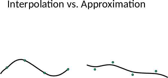
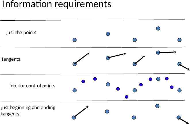
Choosing an interpolating function Tradeoffs and commonly chosen options Interpolation vs. approximation Polynomial complexity: cubic Continuity: first degree (tangential) Local vs. global control: local Information requirements: tangents needed?
Interpolation vs. Approximation
Polynomial complexity Low complexity reduced computational cost With a point of inflection, the curve can match arbitrary tangents at end points Therefore, choose a cubic polynomial
Continuity orders C-1 discontinuous C1 first derivative is continuous C0 continuous C2 first and second derivatives are continuous
Local vs. Global control
Information requirements just the points tangents interior control points just beginning and ending tangents
Curve Formulations General solution – Lagrange Polynomial Piecewise cubic polynomials – Catmull-Rom – Bezier
Lagrange Polynomial x x xk Pj ( x) y j k 1 x j xk k j See http://mathworld.wolfram.com/LagrangeInterpolatingPolynomial.html for more details
Lagrange Polynomial x x xk Pj ( x) y j k 1 x j xk k j Written explicitly term by term is:
Lagrange Polynomial Results are not always good for animation
Polynomial curve formation Generic cubic equation P(u) c3u3 c2u2 c1u c0 u is a parameter that varies from 0 to 1 – u 0 is the first point on the curve – u 1 is the last point on the curve Reminder: our desired output, P, is a vector – c3, c2, c1, and c0 are not scalar values, but vectors – u, as shown above, is a scalar
Polynomial curve formation P(u) c3u3 c2u2 c1u c0 The point P(u) (x(u), y(u), z(u)) where x(u) c3xu3 c2xu2 c1xu c0x y(u) c3yu3 c2yu2 c1yu c0y z(u) c3zu3 c2zu2 c1zu c0z
Polynomial Curve Formulation Matrix multiplication The point at “time” u T P U MB u 3 u2 u 1 Where u is a scalar value in [0,1] Geometric information (i.e. points and/or tangents) Coefficient matrix (given by what curve formulation you are using)
u should be the only variable So how do we set c3, c2, c1, and c0? Or, equivalently, the matrices M and B?
Catmull-Rom spline Passes through control points Tangent at each point pi is based on the previous and next points: (pi 1 pi 1) – Not properly defined at start and end Use a toroidal mapping (lab 5 ; boardwork example) Duplicate the first and last points
Catmull-Rom spline derivation τ is a parameter for tension
Catmull-Rom spline derivation
Catmull-Rom spline derivation Remember: - p( ) is a point - c values are vectors - τ is a constant Use with cubic equation
Catmull-Rom spline derivation Solve for c values in terms of control points
Catmull-Rom matrix form Set τ to 0.5 and put into matrix form P(u ) u 3 u 2 u 1 * 0.5 1.5 1.5 0.5 pi 2 1 2.5 2 0.5 pi 1 * 0.5 0 0.5 0 pi 0 1 0 0 pi 1
Blended Parabolas/Catmull-Rom* Visual example P(u ) u 3 u 2 u 1 * 0.5 1.5 1.5 2.5 2 0.5 0 0.5 0 1 0 1 0.5 pi 2 0.5 pi 1 * 0 pi 0 pi 1 * End conditions are handled differently (or assume curve starts at P1 and stops at Pn-2)
Boardwork example – multiple linear segments or Catmull-Rom splines
Bezier Curve p1 p0 Find the point x on the curve as a function of parameter u: x(u) p2 p3
de Casteljau Algorithm Describe the curve as a recursive series of linear interpolations Intuitive, but not the most efficient form
de Casteljau Algorithm p1 p0 p2 Cubic Bezier curve has four points (though the algorithm works with any number of points) p3
de Casteljau Algorithm p1 q1 q0 p0 p2 q2 q 0 Lerp u, p 0 , p1 q1 Lerp u, p1 , p 2 q 2 Lerp u, p 2 , p 3 Lerp linear interpolation p3
de Casteljau Algorithm q0 r0 q1 r1 q2 r0 Lerp u, q 0 , q1 r1 Lerp u , q1 , q 2
de Casteljau Algorithm r0 x x Lerp u, r0 , r1 r1
Bezier Curve p1 p0 x p2 p3
Cubic Bezier P u3 u2 1.0 3.0 3.0 3.0 6.0 3.0 u 1 3.0 3.0 0.0 0.0 0.0 1.0 Curve runs through Pi and Pi 3 with starting tangent PiPi 1 and ending tangent Pi 2Pi 3 1.0 pi 0.0 pi 1 0.0 pi 2 0.0 pi 3
Controlling Motion along p P(u) Step 1. vary u from 0 to 1 create points on the curve p P(u) But segments may not have equal length Step 2. Reparameterization by arc length u U(s) where s is distance along the curve Step 3. Speed control for example, ease-in / ease-out s ease(t) where t is time
Reparameterizing by Arc Length Analytic Forward differencing Supersampling Adaptive approach Numerically Adaptive Gaussian
Reparameterizing by Arc Length - supersample 1.Calculate a bunch of points at small increments in u 2.Compute summed linear distances as approximation to arc length 3.Build table of (parametric value, arc length) pairs Notes 1.Often useful to normalize total distance to 1.0 2.Often useful to normalize parametric value for multisegment curve to 1.0
Boardwork example – normalizing for multiple linear segments
Supersampling – table of values index u Arc Length (s) 0 0 0 1 0.5 2 2 1 4 3 0 4 4 0.5 10 5 1 16
Supersampling – table of normalized values index u Arc Length (s) 0 0.00 0.000 1 0.05 0.075 2 0.10 0.150 3 0.15 0.230 . . . 20 1.00 1.000
Other possible table data index Segment number u Arc Length (s) 0.000 0 0 0 1 0 2 Point location (x,y,z) 0.5 0.075 (x,y,z) 0 1 0.150 (x,y,z) 3 1 0 0.150 (x,y,z) 4 1 0.5 0.575 (x,y,z) 5 1 1 1.000 (x,y,z)
Speed Control distance Time-distance function Ease-in Ease-out Sinusoidal Cubic polynomial Constant acceleration General distance-time functions time
Time Distance Function S s s S(t) t the global time variable
Ease-in/Ease-out Function s S 1.0 s S(t) 0.0 0.0 1.0 t Normalize distance and time to 1.0 to facilitate reuse
Ease-in: Sinusoidal s ease(t ) sin( t / 2 1) / 2
Ease-in: Single Cubic 3 s ease(t ) 2t 3t 2
Ease-in: Constant Acceleration
Ease-in: Constant Acceleration
Ease-in: Constant Acceleration
Ease-in: Constant Acceleration
Motion on a curve – solution steps 1. Construct a space curve that interpolates the given points with piecewise first order continuity p P(u) 2. Construct an arc-length-parametric-value function for the curve u U(s) 3. Construct time-arc-length function according to given constraints s S(t) p P(U(S(t)))
Arbitrary Speed Control Animators can work in: Distance-time space curves Velocity-time space curves Acceleration-time space curves Set time-distance constraints
References Images from http:// www.cambridgeincolour.com/tutorials/imageinterpolation.htm http:// mathworld.wolfram.com/LagrangeInterpolatin gPolynomial.html
ADDITIONAL SLIDES
Bilinear vs. bicubic interpolation Higher order interpolation requires more sample points