Module 32: Multiple Regression This module reviews simple
46 Slides280.50 KB
Module 32: Multiple Regression This module reviews simple linear regression and then discusses multiple regression. The next module contains several examples Reviewed 19 July 05/MODULE 32
Module Content A. Review of Simple Linear Regression B. Multiple Regression C. Relationship to ANOVA and Analysis of Covariance
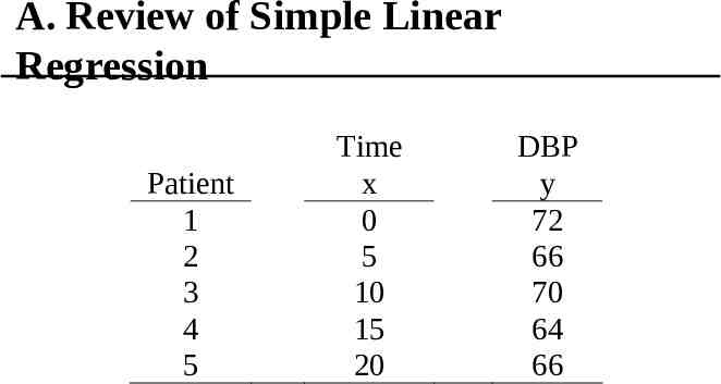
A. Review of Simple Linear Regression Patient 1 2 3 4 5 Time x 0 5 10 15 20 DBP y 72 66 70 64 66
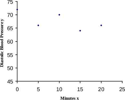
75 Diastolic Blood Pressure y 70 65 60 55 50 45 0 5 10 15 Minutes x 20 25
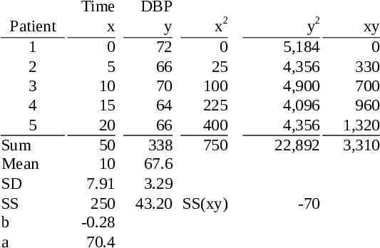
Patient 1 2 3 4 5 Sum Mean SD SS b a Time x 0 5 10 15 20 50 10 7.91 250 -0.28 70.4 DBP y x2 72 0 66 25 70 100 64 225 66 400 338 750 67.6 3.29 43.20 SS(xy) y2 5,184 4,356 4,900 4,096 4,356 22,892 -70 xy 0 330 700 960 1,320 3,310
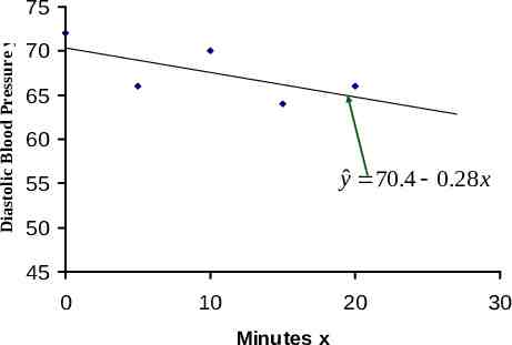
Diastolic Blood Pressure y 75 70 65 60 yˆ 70.4 0.28 x 55 50 45 0 10 20 Minutes x 30
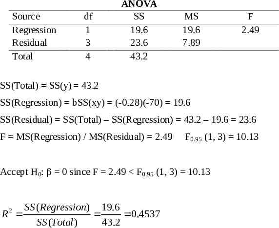
Source Regression Residual Total df 1 3 4 ANOVA SS 19.6 23.6 43.2 MS 19.6 7.89 F 2.49 SS(Total) SS(y) 43.2 SS(Regression) bSS(xy) (-0.28)(-70) 19.6 SS(Residual) SS(Total) – SS(Regression) 43.2 – 19.6 23.6 F MS(Regression) / MS(Residual) 2.49 F0.95 (1, 3) 10.13 Accept H0: 0 since F 2.49 F0.95 (1, 3) 10.13 SS ( Regression) 19.6 R 0.4537 SS (Total ) 43.2 2
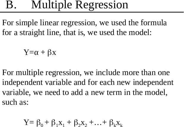
B. Multiple Regression For simple linear regression, we used the formula for a straight line, that is, we used the model: Y α x For multiple regression, we include more than one independent variable and for each new independent variable, we need to add a new term in the model, such as: Y 0 1x1 2x2 kxk
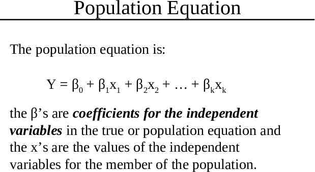
Population Equation The population equation is: Y β0 β1x1 β2x2 βkxk the β’s are coefficients for the independent variables in the true or population equation and the x’s are the values of the independent variables for the member of the population.
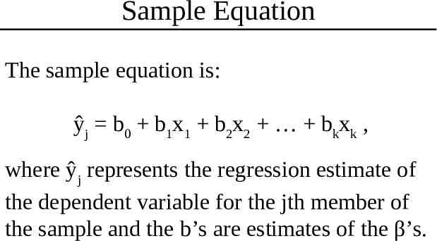
Sample Equation The sample equation is: ŷj b0 b1x1 b2x2 bkxk , where ŷj represents the regression estimate of the dependent variable for the jth member of the sample and the b’s are estimates of the β’s.
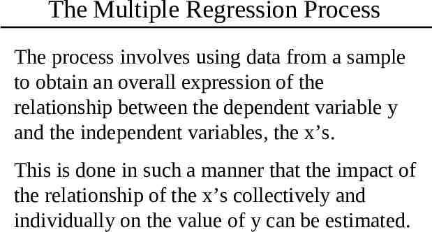
The Multiple Regression Process The process involves using data from a sample to obtain an overall expression of the relationship between the dependent variable y and the independent variables, the x’s. This is done in such a manner that the impact of the relationship of the x’s collectively and individually on the value of y can be estimated.
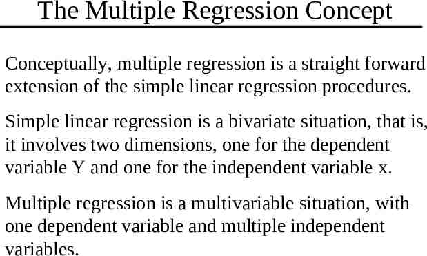
The Multiple Regression Concept Conceptually, multiple regression is a straight forward extension of the simple linear regression procedures. Simple linear regression is a bivariate situation, that is, it involves two dimensions, one for the dependent variable Y and one for the independent variable x. Multiple regression is a multivariable situation, with one dependent variable and multiple independent variables.
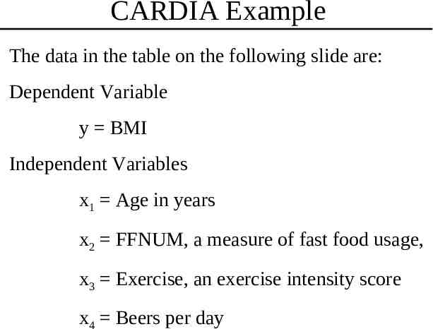
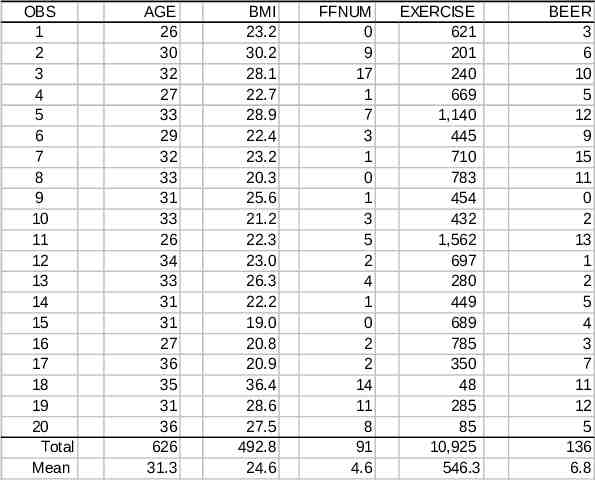
CARDIA Example The data in the table on the following slide are: Dependent Variable y BMI Independent Variables x1 Age in years x2 FFNUM, a measure of fast food usage, x3 Exercise, an exercise intensity score x4 Beers per day
OBS 1 2 3 4 5 6 7 8 9 10 11 12 13 14 15 16 17 18 19 20 Total Mean AGE 26 30 32 27 33 29 32 33 31 33 26 34 33 31 31 27 36 35 31 36 626 31.3 BMI 23.2 30.2 28.1 22.7 28.9 22.4 23.2 20.3 25.6 21.2 22.3 23.0 26.3 22.2 19.0 20.8 20.9 36.4 28.6 27.5 492.8 24.6 FFNUM 0 9 17 1 7 3 1 0 1 3 5 2 4 1 0 2 2 14 11 8 91 4.6 EXERCISE 621 201 240 669 1,140 445 710 783 454 432 1,562 697 280 449 689 785 350 48 285 85 10,925 546.3 BEER 3 6 10 5 12 9 15 11 0 2 13 1 2 5 4 3 7 11 12 5 136 6.8
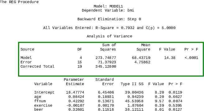
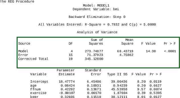
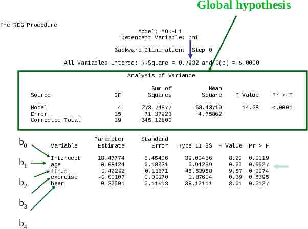
The REG Procedure Model: MODEL1 Dependent Variable: bmi Backward Elimination: Step 0 All Variables Entered: R-Square 0.7932 and C(p) 5.0000 Analysis of Variance Source DF Sum of Squares Model Error Corrected Total 4 15 19 273.74877 71.37923 345.12800 Variable Intercept age ffnum exercise beer Mean Square 68.43719 4.75862 F Value Pr F 14.38 .0001 Parameter Estimate Standard Error Type II SS F Value Pr F 18.47774 0.08424 0.42292 -0.00107 0.32601 6.45406 0.18931 0.13671 0.00170 0.11518 39.00436 0.94239 45.53958 1.87604 38.12111 8.20 0.20 9.57 0.39 8.01 0.0119 0.6627 0.0074 0.5395 0.0127
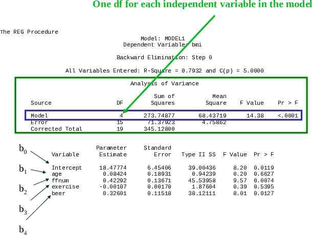
One df for each independent variable in the model The REG Procedure Model: MODEL1 Dependent Variable: bmi Backward Elimination: Step 0 All Variables Entered: R-Square 0.7932 and C(p) 5.0000 Analysis of Variance b0 b1 b2 b3 b4 Source DF Sum of Squares Mean Square Model Error Corrected Total 4 15 19 273.74877 71.37923 345.12800 68.43719 4.75862 F Value Pr F 14.38 .0001 Variable Parameter Estimate Standard Error Type II SS F Value Pr F Intercept age ffnum exercise beer 18.47774 0.08424 0.42292 -0.00107 0.32601 6.45406 0.18931 0.13671 0.00170 0.11518 39.00436 0.94239 45.53958 1.87604 38.12111 8.20 0.20 9.57 0.39 8.01 0.0119 0.6627 0.0074 0.5395 0.0127
The REG Procedure Model: MODEL1 Dependent Variable: bmi Backward Elimination: Step 0 All Variables Entered: R-Square 0.7932 and C(p) 5.0000 Analysis of Variance Source DF Sum of Squares Model Error Corrected Total 4 15 19 273.74877 71.37923 345.12800 b0 b1 b2 b3 b4 Variable Intercept age ffnum exercise beer Mean Square 68.43719 4.75862 F Value Pr F 14.38 .0001 Parameter Estimate Standard Error Type II SS F Value Pr F 18.47774 0.08424 0.42292 -0.00107 0.32601 6.45406 0.18931 0.13671 0.00170 0.11518 39.00436 0.94239 45.53958 1.87604 38.12111 8.20 0.20 9.57 0.39 8.01 0.0119 0.6627 0.0074 0.5395 0.0127
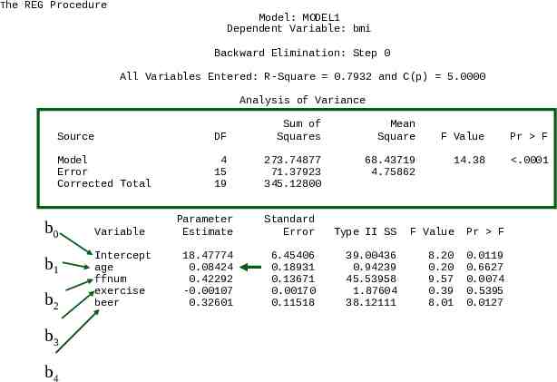
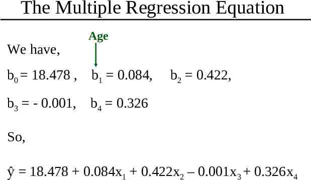
The Multiple Regression Equation We have, Age b0 18.478 , b1 0.084, b2 0.422, b3 - 0.001, b4 0.326 So, ŷ 18.478 0.084x1 0.422x2 – 0.001x3 0.326x4
The Multiple Regression Coefficient The interpretation of the multiple regression coefficient is similar to that for the simple linear regression coefficient, except that the phrase “adjusted for the other terms in the model” should be added. For example, the coefficient for Age in the model is b1 0.084, for which the interpretation is that for every unit increase in age, that is for every one year increase in age, the BMI goes up 0.084 units, adjusted for the other three terms in the model.
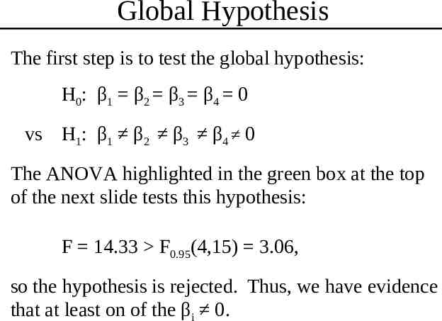
Global Hypothesis The first step is to test the global hypothesis: H0: β1 β2 β3 β4 0 vs H1: β1 β2 β3 β4 0 The ANOVA highlighted in the green box at the top of the next slide tests this hypothesis: F 14.33 F0.95(4,15) 3.06, so the hypothesis is rejected. Thus, we have evidence that at least on of the βi 0.
The REG Procedure Model: MODEL1 Dependent Variable: bmi Backward Elimination: Step 0 All Variables Entered: R-Square 0.7932 and C(p) 5.0000 Analysis of Variance Source DF Sum of Squares Model Error Corrected Total 4 15 19 273.74877 71.37923 345.12800 Variable Intercept age ffnum exercise beer Mean Square 68.43719 4.75862 F Value Pr F 14.38 .0001 Parameter Estimate Standard Error Type II SS F Value Pr F 18.47774 0.08424 0.42292 -0.00107 0.32601 6.45406 0.18931 0.13671 0.00170 0.11518 39.00436 0.94239 45.53958 1.87604 38.12111 8.20 0.20 9.57 0.39 8.01 0.0119 0.6627 0.0074 0.5395 0.0127
Variation in BMI Explained by Model The amount of variation in the dependent variable, BMI, explained by its regression relationship with the four independent variables is R2 SS(Model)/SS(Total) 273.75/345.13 0.79 or 79%
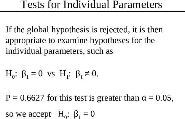
Tests for Individual Parameters If the global hypothesis is rejected, it is then appropriate to examine hypotheses for the individual parameters, such as H0: β1 0 vs H1: β1 0. P 0.6627 for this test is greater than α 0.05, so we accept H0: β1 0
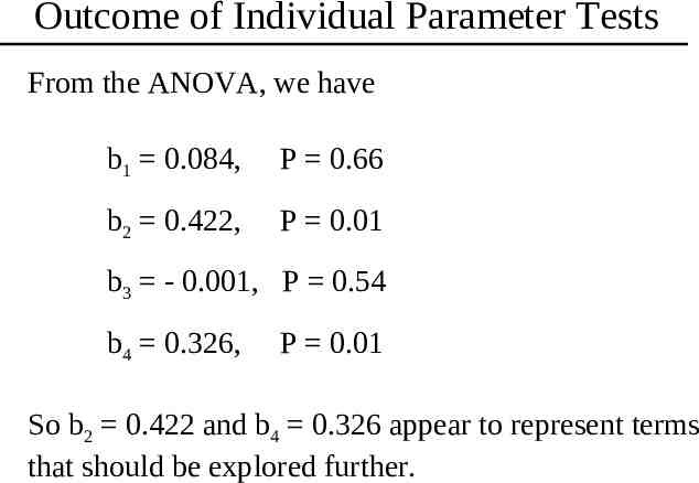
Outcome of Individual Parameter Tests From the ANOVA, we have b1 0.084, P 0.66 b2 0.422, P 0.01 b3 - 0.001, P 0.54 b4 0.326, P 0.01 So b2 0.422 and b4 0.326 appear to represent terms that should be explored further.
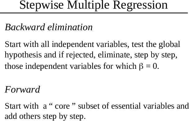
Stepwise Multiple Regression Backward elimination Start with all independent variables, test the global hypothesis and if rejected, eliminate, step by step, those independent variables for which 0. Forward Start with a “ core ” subset of essential variables and add others step by step.
Backward Elimination The next few slides show the process and steps for the backward elimination procedure.
Global hypothesis The REG Procedure Model: MODEL1 Dependent Variable: bmi Backward Elimination: Step 0 All Variables Entered: R-Square 0.7932 and C(p) 5.0000 Analysis of Variance b0 b1 b2 b3 b4 Source DF Sum of Squares Mean Square Model Error Corrected Total 4 15 19 273.74877 71.37923 345.12800 68.43719 4.75862 Variable Intercept age ffnum exercise beer F Value Pr F 14.38 .0001 Parameter Estimate Standard Error Type II SS F Value Pr F 18.47774 0.08424 0.42292 -0.00107 0.32601 6.45406 0.18931 0.13671 0.00170 0.11518 39.00436 0.94239 45.53958 1.87604 38.12111 8.20 0.20 9.57 0.39 8.01 0.0119 0.6627 0.0074 0.5395 0.0127
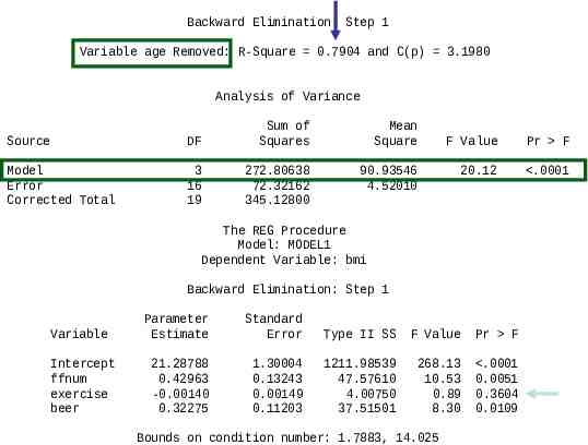
Backward Elimination: Step 1 Variable age Removed: R-Square 0.7904 and C(p) 3.1980 Analysis of Variance Source DF Sum of Squares Mean Square Model Error Corrected Total 3 16 19 272.80638 72.32162 345.12800 90.93546 4.52010 F Value Pr F 20.12 .0001 The REG Procedure Model: MODEL1 Dependent Variable: bmi Backward Elimination: Step 1 Variable Parameter Estimate Standard Error Type II SS F Value Pr F Intercept ffnum exercise beer 21.28788 0.42963 -0.00140 0.32275 1.30004 0.13243 0.00149 0.11203 1211.98539 47.57610 4.00750 37.51501 268.13 10.53 0.89 8.30 .0001 0.0051 0.3604 0.0109 Bounds on condition number: 1.7883, 14.025
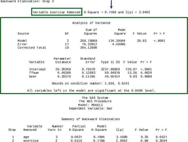
Backward Elimination: Step 2 Variable exercise Removed: R-Square 0.7788 and C(p) 2.0402 Analysis of Variance Source DF Sum of Squares Mean Square Model Error Corrected Total 2 17 19 268.79888 76.32912 345.12800 134.39944 4.48995 Variable Intercept ffnum beer F Value Pr F 29.93 .0001 Parameter Estimate Standard Error Type II SS F Value Pr F 20.29360 0.46380 0.33375 0.75579 0.12693 0.11105 3237.09859 59.94878 40.55414 720.97 13.35 9.03 .0001 0.0020 0.0080 Bounds on condition number: 1.654, 6.6161 All variables left in the model are significant at the 0.0500 level. The SAS System The REG Procedure Model: MODEL1 Dependent Variable: bmi Summary of Backward Elimination Step 1 2 Variable Removed age exercise Number Vars In Partial R-Square Model R-Square 3 2 0.0027 0.0116 0.7904 0.7788 C(p) 3.1980 2.0402 F Value Pr F 0.20 0.89 0.6627 0.3604
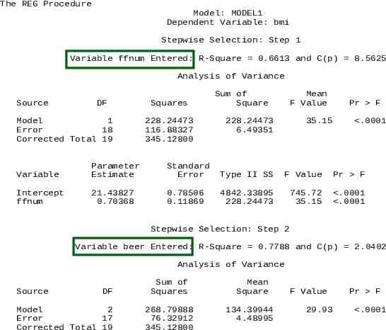
Forward Stepwise Regression The next two slides show the process and steps for Forward Stepwise Regression. In this procedure, the first independent variable entered into the model is the one with the highest correlation with the dependent variable.
The REG Procedure Model: MODEL1 Dependent Variable: bmi Stepwise Selection: Step 1 Variable ffnum Entered: R-Square 0.6613 and C(p) 8.5625 Analysis of Variance Source DF Model 1 Error 18 Corrected Total 19 Squares 228.24473 116.88327 345.12800 Sum of Square Mean F Value 228.24473 6.49351 35.15 Pr F .0001 Variable Parameter Estimate Standard Error Type II SS F Value Pr F Intercept ffnum 21.43827 0.70368 0.78506 0.11869 4842.33895 228.24473 745.72 35.15 .0001 .0001 Stepwise Selection: Step 2 Variable beer Entered: R-Square 0.7788 and C(p) 2.0402 Analysis of Variance Source DF Model 2 Error 17 Corrected Total 19 Sum of Squares 268.79888 76.32912 345.12800 Mean Square 134.39944 4.48995 F Value 29.93 Pr F .0001
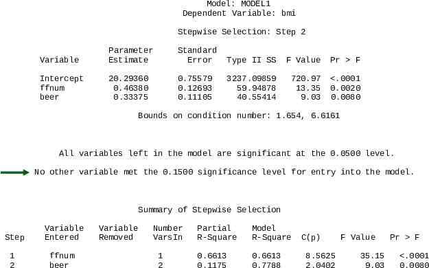
Model: MODEL1 Dependent Variable: bmi Stepwise Selection: Step 2 Variable Parameter Estimate Standard Error Type II SS F Value Pr F Intercept ffnum beer 20.29360 0.46380 0.33375 0.75579 0.12693 0.11105 3237.09859 59.94878 40.55414 720.97 13.35 9.03 .0001 0.0020 0.0080 Bounds on condition number: 1.654, 6.6161 All variables left in the model are significant at the 0.0500 level. No other variable met the 0.1500 significance level for entry into the model. Summary of Stepwise Selection Step Variable Entered 1 2 ffnum beer Variable Removed Number VarsIn 1 2 Partial R-Square Model R-Square 0.6613 0.1175 0.6613 0.7788 C(p) 8.5625 2.0402 F Value 35.15 9.03 Pr F .0001 0.0080
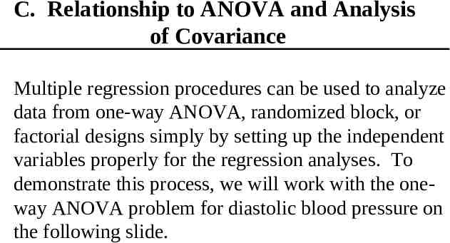
C. Relationship to ANOVA and Analysis of Covariance Multiple regression procedures can be used to analyze data from one-way ANOVA, randomized block, or factorial designs simply by setting up the independent variables properly for the regression analyses. To demonstrate this process, we will work with the oneway ANOVA problem for diastolic blood pressure on the following slide.
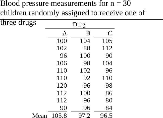
Blood pressure measurements for n 30 children randomly assigned to receive one of three drugs Drug A 100 102 96 106 110 110 120 112 112 90 Mean 105.8 B 104 88 100 98 102 92 96 100 96 96 97.2 C 105 112 90 104 96 110 98 86 80 84 96.5
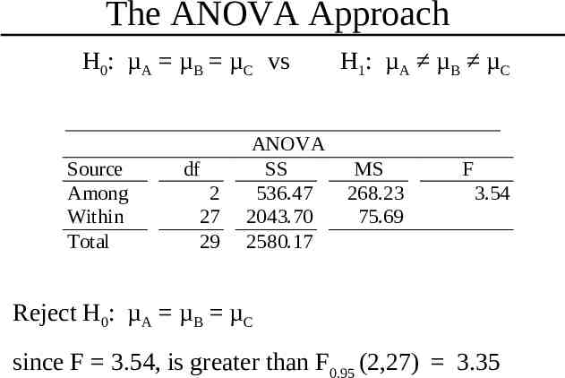
The ANOVA Approach H0: µA µB µC vs Source Among Within Total df 2 27 29 ANOVA SS 536.47 2043.70 2580.17 H1: µA µB µC MS 268.23 75.69 F 3.54 Reject H0: µA µB µC since F 3.54, is greater than F0.95 (2,27) 3.35
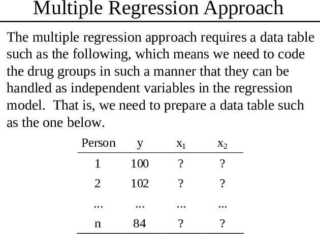
Multiple Regression Approach The multiple regression approach requires a data table such as the following, which means we need to code the drug groups in such a manner that they can be handled as independent variables in the regression model. That is, we need to prepare a data table such as the one below. Person y x1 x2 1 100 ? ? 2 102 ? ? . . . . n 84 ? ?
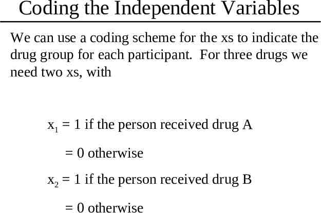
Coding the Independent Variables We can use a coding scheme for the xs to indicate the drug group for each participant. For three drugs we need two xs, with x1 1 if the person received drug A 0 otherwise x2 1 if the person received drug B 0 otherwise
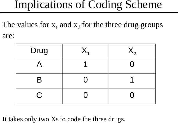
Implications of Coding Scheme The values for x1 and x2 for the three drug groups are: Drug X1 X2 A 1 0 B 0 1 C 0 0 It takes only two Xs to code the three drugs.
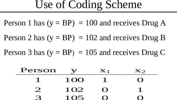
Use of Coding Scheme Person 1 has (y BP) 100 and receives Drug A Person 2 has (y BP) 102 and receives Drug B Person 3 has (y BP) 105 and receives Drug C Person 1 2 3 y 100 102 105 x1 1 0 0 x2 0 1 0
Indicator Variables These “indicator” variables provide a mechanism for including categories into analyses using multiple regression techniques. If they are used properly, they can be made to represent complex study designs. Adding such variables to a multiple regression analysis is readily accomplished. For proper interpretation, one needs to keep in mind how the different variables are defined; otherwise, the process is straight forward multiple regression.
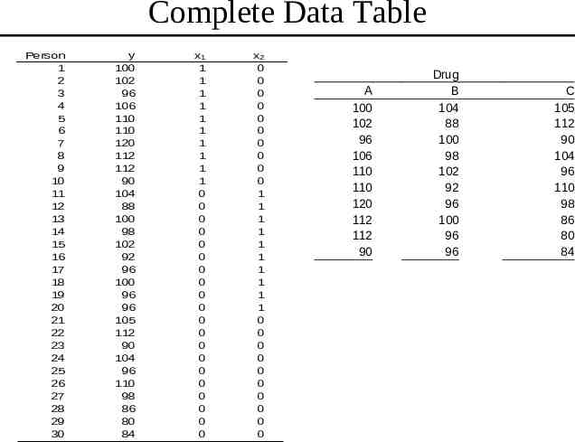
Complete Data Table Person 1 2 3 4 5 6 7 8 9 10 11 12 13 14 15 16 17 18 19 20 21 22 23 24 25 26 27 28 29 30 y 100 102 96 106 110 110 120 112 112 90 104 88 100 98 102 92 96 100 96 96 105 112 90 104 96 110 98 86 80 84 x1 1 1 1 1 1 1 1 1 1 1 0 0 0 0 0 0 0 0 0 0 0 0 0 0 0 0 0 0 0 0 x2 0 0 0 0 0 0 0 0 0 0 1 1 1 1 1 1 1 1 1 1 0 0 0 0 0 0 0 0 0 0 A 100 102 96 106 110 110 120 112 112 90 Drug B 104 88 100 98 102 92 96 100 96 96 C 105 112 90 104 96 110 98 86 80 84
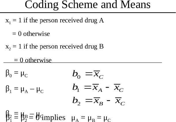
Coding Scheme and Means x1 1 if the person received drug A 0 otherwise x2 1 if the person received drug B 0 otherwise β0 μC b0 xC β1 μA – μC b1 x A xC b2 xB xC ββ2 μ – 0μCimplies μ μ μ B β 1 2 A B C
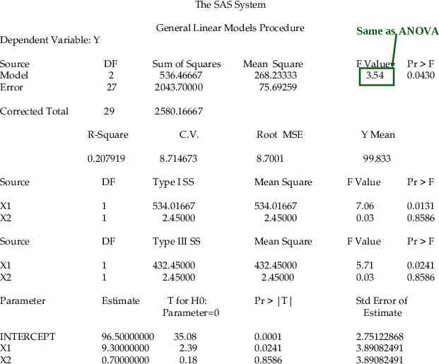
The SAS System General Linear Models Procedure Dependent Variable: Y Source Model Error DF 2 27 Sum of Squares 536.46667 2043.70000 Corrected Total 29 2580.16667 R-Square C.V. 0.207919 8.714673 Mean Square 268.23333 75.69259 Y Mean 8.7001 99.833 DF Type I SS Mean Square X1 X2 1 1 534.01667 2.45000 534.01667 2.45000 Source DF Type III SS Mean Square X1 X2 1 1 432.45000 2.45000 Parameter Estimate INTERCEPT X1 X2 96.50000000 9.30000000 0.70000000 35.08 2.39 0.18 F Value 3.54 Root MSE Source T for H0: Parameter 0 Same as ANOVA Pr F 0.0430 F Value Pr F 7.06 0.03 0.0131 0.8586 F Value Pr F 432.45000 2.45000 5.71 0.03 0.0241 0.8586 Pr T Std Error of Estimate 0.0001 0.0241 0.8586 2.75122868 3.89082491 3.89082491
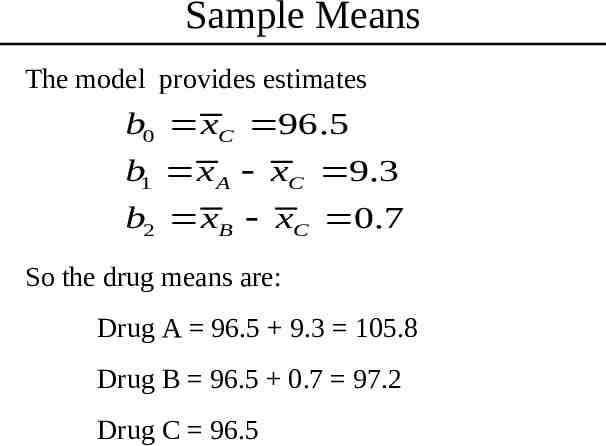
Sample Means The model provides estimates b0 xC 96.5 b1 x A xC 9.3 b2 xB xC 0.7 So the drug means are: Drug A 96.5 9.3 105.8 Drug B 96.5 0.7 97.2 Drug C 96.5
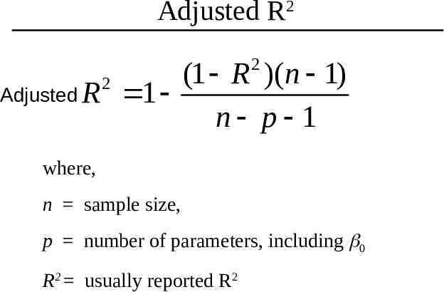
Adjusted R2 2 (1 R )(n 1) Adjusted R 1 n p 1 2 where, n sample size, p number of parameters, including 0 R2 usually reported R2
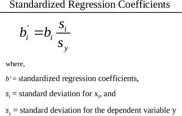
Standardized Regression Coefficients si b bi sy ' i where, b' standardized regression coefficients, si standard deviation for xi, and sy standard deviation for the dependent variable y