Chapter 2 Frequency Distributions and Graphs Section 2-2


45 Slides729.50 KB
Chapter 2 Frequency Distributions and Graphs Section 2-2 Organizing Data
Chapter 2 Frequency Distributions and Graphs Section 2-2 Exercise #7
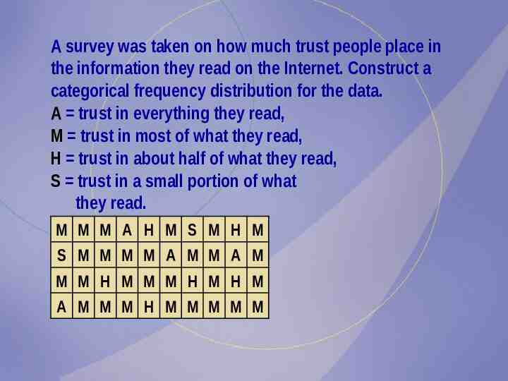
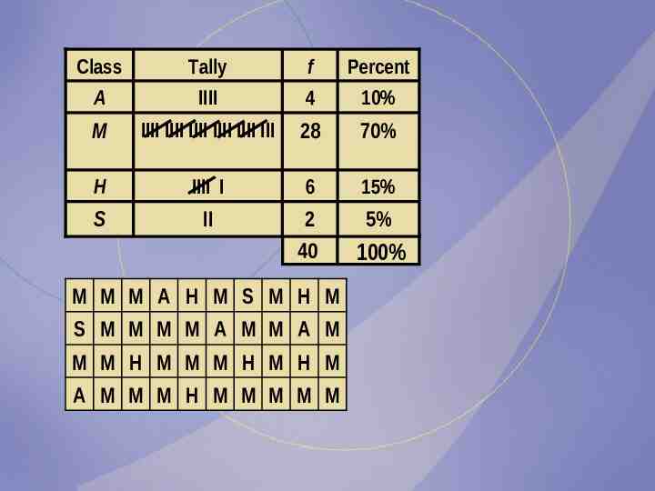
A survey was taken on how much trust people place in the information they read on the Internet. Construct a categorical frequency distribution for the data. A trust in everything they read, M trust in most of what they read, H trust in about half of what they read, S trust in a small portion of what they read. M M M A H M S M H M S M M M M A M M A M M M H M M M H M H M A M M M H M M M M M
Class Tally f Percent A IIII 4 10% M IIII IIII IIII IIII IIII III 28 70% H IIII I 6 15% S II 2 40 5% M M M A H M S M H M S M M M M A M M A M M M H M M M H M H M A M M M H M M M M M 100%
Chapter 2 Frequency Distributions and Graphs Section 2-2 Exercise #11
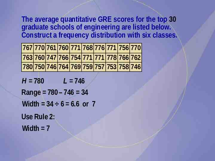
The average quantitative GRE scores for the top 30 graduate schools of engineering are listed below. Construct a frequency distribution with six classes. 767 770 761 760 771 768 776 771 756 770 763 760 747 766 754 771 771 778 766 762 780 750 746 764 769 759 757 753 758 746 H 780 L 746 Range 780 – 746 34 Width 34 6 6.6 or 7 Use Rule 2: Width 7
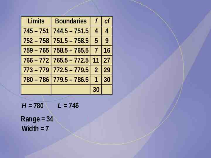
Limits 745 – 751 752 – 758 759 – 765 766 – 772 773 – 779 780 – 786 H 780 Range 34 Width 7 Boundaries 744.5 – 751.5 751.5 – 758.5 758.5 – 765.5 765.5 – 772.5 772.5 – 779.5 779.5 – 786.5 L 746 f 4 5 7 11 2 1 30 cf 4 9 16 27 29 30
Chapter 2 Frequency Distributions and Graphs Section 2-2 Exercise #13
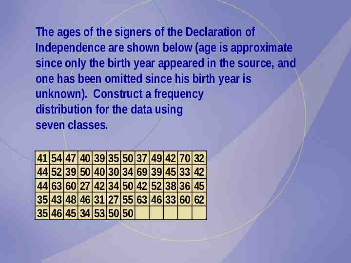
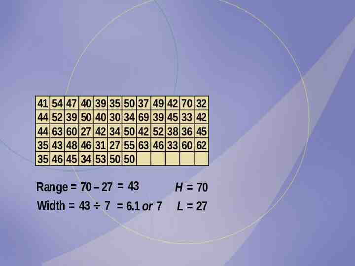
The ages of the signers of the Declaration of Independence are shown below (age is approximate since only the birth year appeared in the source, and one has been omitted since his birth year is unknown). Construct a frequency distribution for the data using seven classes. 41 44 44 35 35 54 52 63 43 46 47 39 60 48 45 40 50 27 46 34 39 40 42 31 53 35 30 34 27 50 50 34 50 55 50 37 69 42 63 49 39 52 46 42 45 38 33 70 33 36 60 32 42 45 62
41 44 44 35 35 54 52 63 43 46 47 39 60 48 45 40 50 27 46 34 39 40 42 31 53 35 30 34 27 50 50 34 50 55 50 37 69 42 63 49 39 52 46 Range 70 – 27 43 Width 43 7 6.1 or 7 42 45 38 33 70 33 36 60 32 42 45 62 H 70 L 27
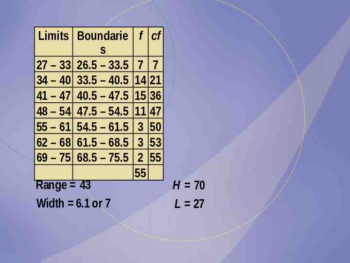
Limits Boundarie s 27 – 33 26.5 – 33.5 34 – 40 33.5 – 40.5 41 – 47 40.5 – 47.5 48 – 54 47.5 – 54.5 55 – 61 54.5 – 61.5 62 – 68 61.5 – 68.5 69 – 75 68.5 – 75.5 Range 43 Width 6.1 or 7 f cf 7 7 14 21 15 36 11 47 3 50 3 53 2 55 55 H 70 L 27
Chapter 2 Frequency Distributions and Graphs Section 2-3 Exercise #1 Histograms, Frequency Polygons, and Ogives
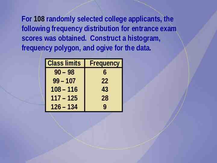
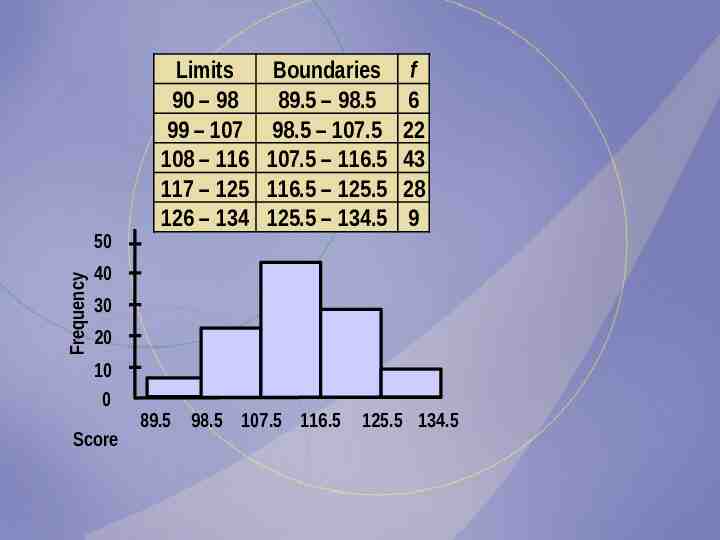
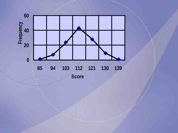
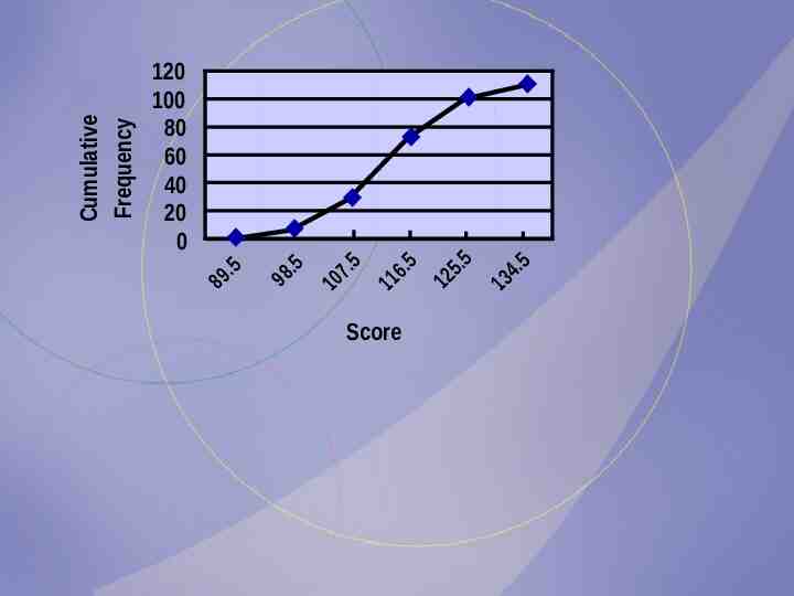
For 108 randomly selected college applicants, the following frequency distribution for entrance exam scores was obtained. Construct a histogram, frequency polygon, and ogive for the data. Class limits 90 – 98 99 – 107 108 – 116 117 – 125 126 – 134 Frequency 6 22 43 28 9
Frequency 50 Limits 90 – 98 99 – 107 108 – 116 117 – 125 126 – 134 Boundaries 89.5 – 98.5 98.5 – 107.5 107.5 – 116.5 116.5 – 125.5 125.5 – 134.5 f 6 22 43 28 9 40 30 20 10 0 Score 89.5 98.5 107.5 116.5 125.5 134.5
Frequency 60 40 20 0 85 94 103 112 Score 121 130 139
98 .5 10 7.5 11 6.5 12 5.5 13 4.5 89 .5 Cumulative Frequency 120 100 80 60 40 20 0 Score
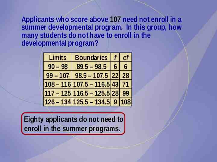
Applicants who score above 107 need not enroll in a summer developmental program. In this group, how many students do not have to enroll in the developmental program? Limits 90 – 98 99 – 107 108 – 116 117 – 125 126 – 134 Boundaries 89.5 – 98.5 98.5 – 107.5 107.5 – 116.5 116.5 – 125.5 125.5 – 134.5 f 6 22 43 28 9 cf 6 28 71 99 108 Eighty applicants do not need to enroll in the summer programs.
Chapter 2 Frequency Distributions and Graphs Section 2-3 Exercise #7 Histograms, Frequency Polygons, and Ogives
The air quality measured for selected cities in the United States for 1993 and 2002 are shown. The data are the number of days per year that the cities failed to meet acceptable standards. Construct a histogram for both years and see if there are any notable changes. If so, explain.
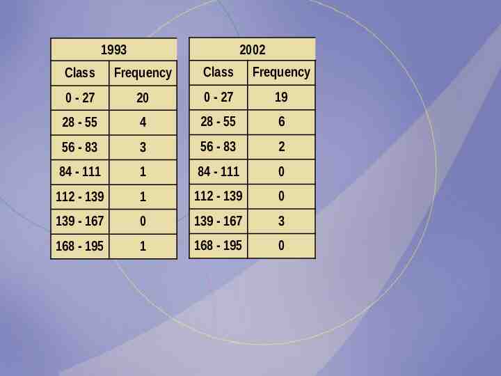
2002 1993 Class Frequency Class Frequency 0 - 27 20 0 - 27 19 28 - 55 4 28 - 55 6 56 - 83 3 56 - 83 2 84 - 111 1 84 - 111 0 112 - 139 1 112 - 139 0 139 - 167 0 139 - 167 3 168 - 195 1 168 - 195 0
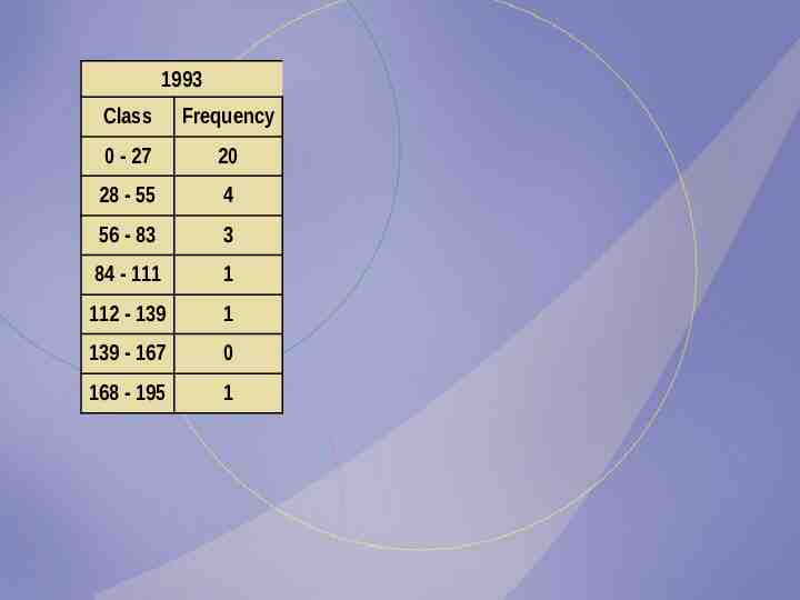
1993 Class Frequency 0 - 27 20 28 - 55 4 56 - 83 3 84 - 111 1 112 - 139 1 139 - 167 0 168 - 195 1
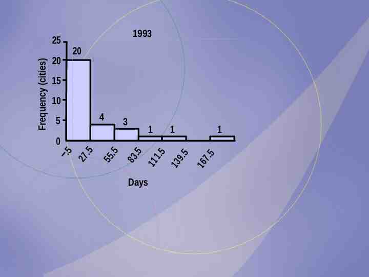
1 Days 16 7.5 3 11 1.5 13 9.5 4 83 .5 5 55 .5 20 27 .5 .5 Frequency (cities) 25 1993 20 15 10 1 1 0
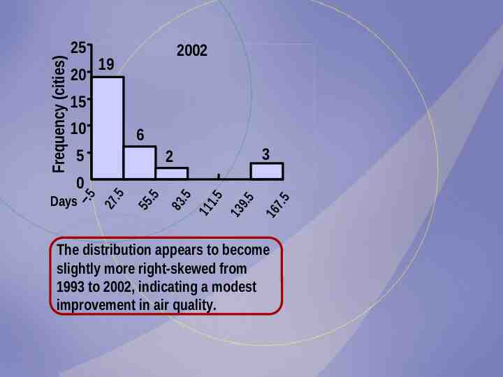
2002 Class Frequency 0 - 27 19 28 - 55 6 56 - 83 2 84 - 111 0 112 - 139 0 139 - 167 3 168 - 195 0
20 2002 19 15 10 6 5 3 2 16 7.5 11 1.5 13 9.5 83 .5 .5 Days 55 .5 0 27 .5 Frequency (cities) 25 The distribution appears to become slightly more right-skewed from 1993 to 2002, indicating a modest improvement in air quality.
Chapter 2 Frequency Distributions and Graphs Section 2-3 Exercise #15 Histograms, Frequency Polygons, and Ogives
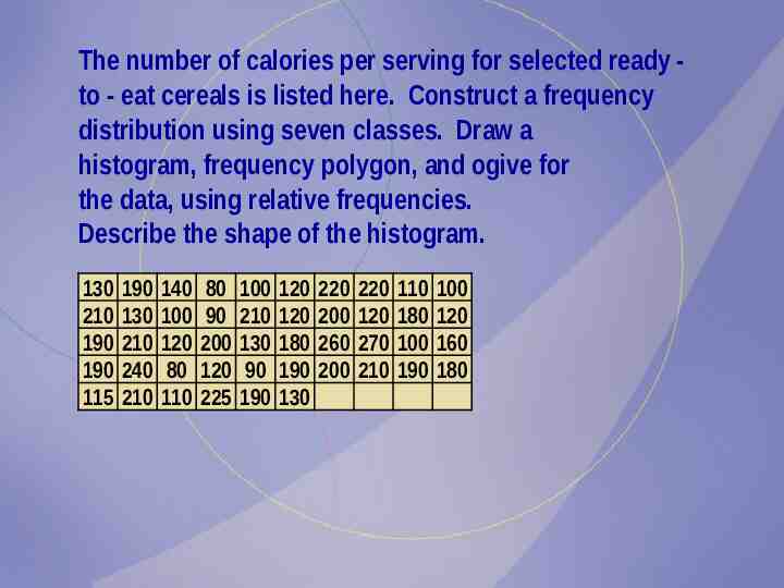
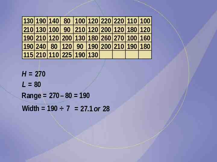
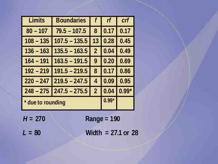
The number of calories per serving for selected ready to - eat cereals is listed here. Construct a frequency distribution using seven classes. Draw a histogram, frequency polygon, and ogive for the data, using relative frequencies. Describe the shape of the histogram. 130 210 190 190 115 190 130 210 240 210 140 100 120 80 110 80 90 200 120 225 100 210 130 90 190 120 120 180 190 130 220 200 260 200 220 120 270 210 110 180 100 190 100 120 160 180
130 210 190 190 115 190 130 210 240 210 140 100 120 80 110 80 90 200 120 225 100 210 130 90 190 120 120 180 190 130 220 200 260 200 H 270 L 80 Range 270 – 80 190 Width 190 7 27.1 or 28 220 120 270 210 110 180 100 190 100 120 160 180
Limits Boundaries f rf crf 80 – 107 79.5 – 107.5 8 0.17 0.17 108 – 135 107.5 – 135.5 13 0.28 0.45 136 – 163 135.5 – 163.5 2 0.04 0.49 164 – 191 163.5 – 191.5 9 0.20 0.69 192 – 219 191.5 – 219.5 8 0.17 0.86 220 – 247 219.5 – 247.5 4 0.09 0.95 248 – 275 247.5 – 275.5 2 0.04 0.99* * due to rounding 0.99* H 270 Range 190 L 80 Width 27.1 or 28
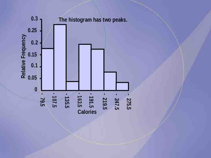
0.3 The histogram has two peaks. Relative Frequency 0.25 0.2 0.15 0.1 0.05 - 275.5 - 247.5 Calories - 219.5 - 191.5 - 135.5 - 107.5 - 79.5 - 163.5 0
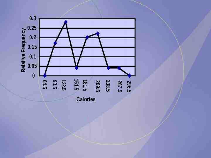
0.25 0.2 0.15 0.1 0.05 296.5 267.5 Calories 238.5 209.5 181.5 64.5 93.5 122.5 151.5 0 Relative Frequency 0.3
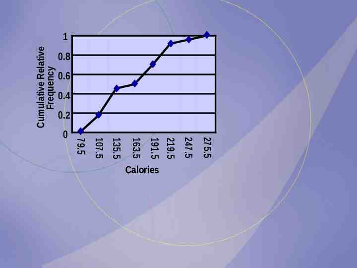
0.8 0.6 0.4 0.2 Cumulative Relative Frequency 1 275.5 247.5 Calories 219.5 191.5 163.5 135.5 107.5 79.5 0
Chapter 2 Frequency Distributions and Graphs Section 2-4 Exercise #1 Other Types of Graphs
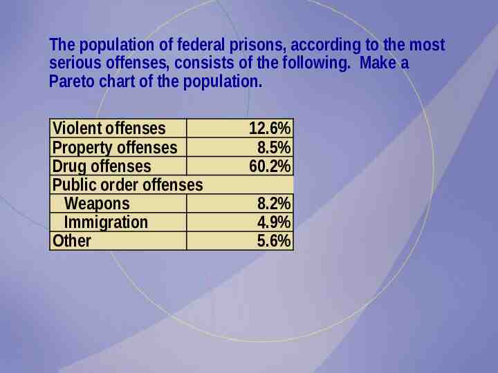
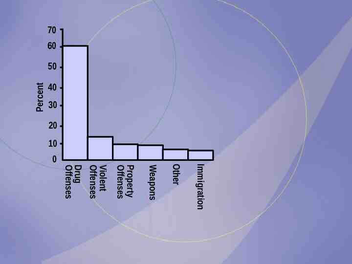
The population of federal prisons, according to the most serious offenses, consists of the following. Make a Pareto chart of the population. Violent offenses Property offenses Drug offenses Public order offenses Weapons Immigration Other 12.6% 8.5% 60.2% 8.2% 4.9% 5.6%
40 30 Percent 70 60 50 20 10 Immigration Drug Offenses Violent Offenses Property Offenses Weapons Other 0
Chapter 2 Frequency Distributions and Graphs Section 2-4 Exercise #7 Other Types of Graphs
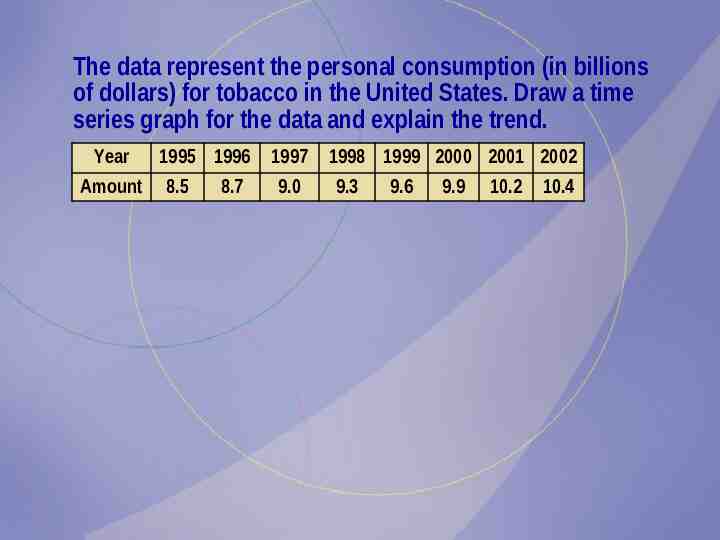
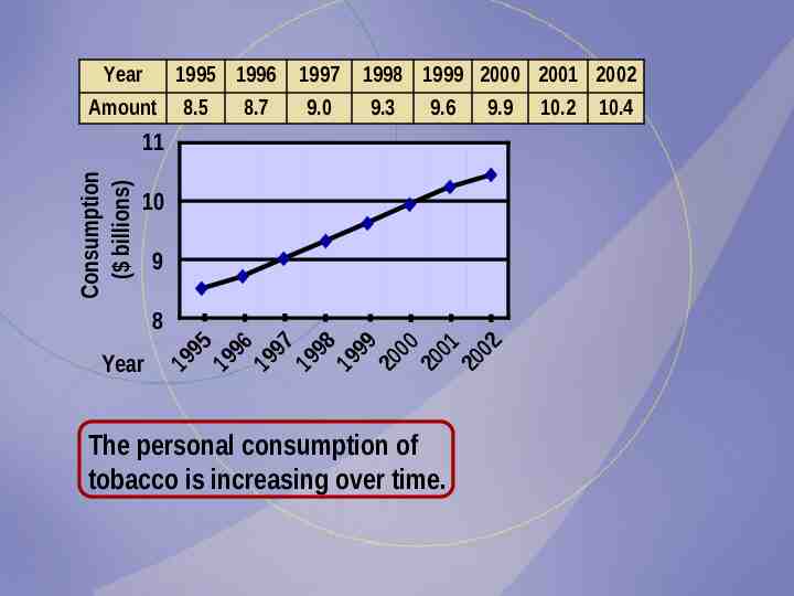
The data represent the personal consumption (in billions of dollars) for tobacco in the United States. Draw a time series graph for the data and explain the trend. Year 1995 1996 Amount 8.5 8.7 1997 9.0 1998 1999 2000 2001 2002 9.3 9.6 9.9 10.2 10.4
Year 1995 1996 Amount 8.5 8.7 1997 9.0 1998 1999 2000 2001 2002 9.3 9.6 9.9 10.2 10.4 Consumption ( billions) 11 10 9 Year 19 95 19 96 19 97 19 98 19 99 20 00 20 01 20 02 8 The personal consumption of tobacco is increasing over time.
Chapter 2 Frequency Distributions and Graphs Section 2-4 Exercise #11 Other Types of Graphs
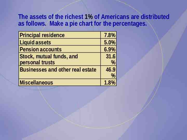
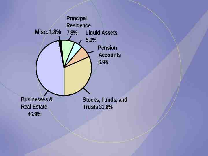
The assets of the richest 1% of Americans are distributed as follows. Make a pie chart for the percentages. Principal residence Liquid assets Pension accounts Stock, mutual funds, and personal trusts Businesses and other real estate Miscellaneous 7.8% 5.0% 6.9% 31.6 % 46.9 % 1.8%
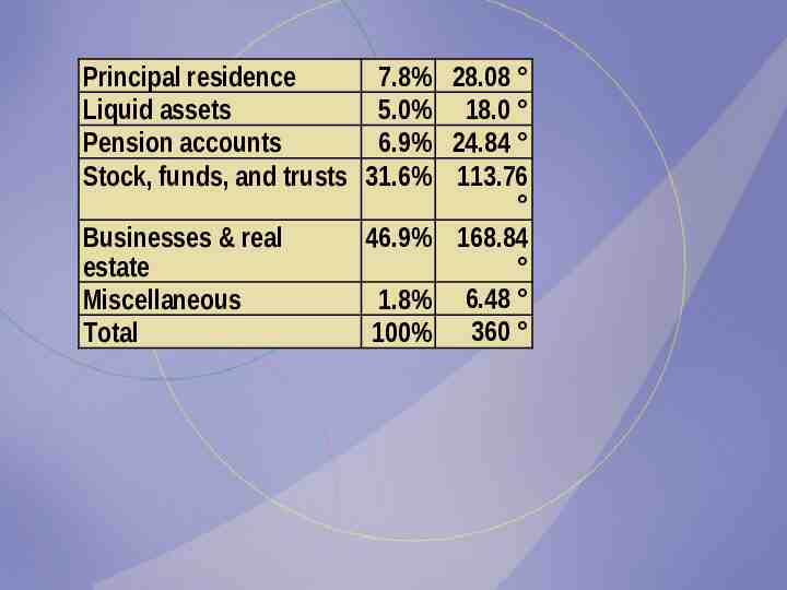
Principal residence 7.8% 28.08 Liquid assets 5.0% 18.0 Pension accounts 6.9% 24.84 Stock, funds, and trusts 31.6% 113.76 Businesses & real 46.9% 168.84 estate Miscellaneous 1.8% 6.48 Total 100% 360
Principal Residence Misc. 1.8% 7.8% Liquid Assets 5.0% Pension Accounts 6.9% Businesses & Real Estate 46.9% Stocks, Funds, and Trusts 31.6%
Chapter 2 Frequency Distributions and Graphs Section 2-4 Exercise #15 Other Types of Graphs
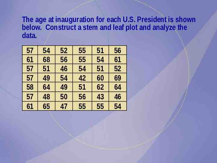
The age at inauguration for each U.S. President is shown below. Construct a stem and leaf plot and analyze the data. 57 61 57 57 58 57 61 54 68 51 49 64 48 65 52 56 46 54 49 50 47 55 55 54 42 51 56 55 51 54 51 60 62 43 55 56 61 52 69 64 46 54
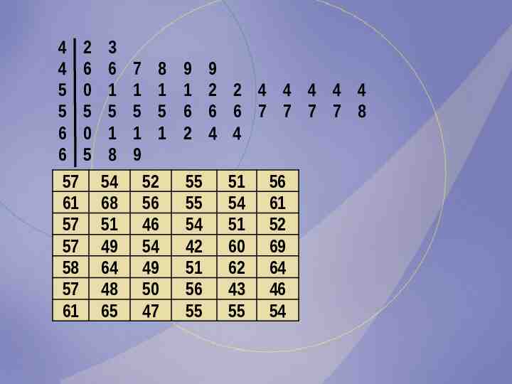
4 2 4 6 5 0 5 5 6 0 6 5 57 61 57 57 58 57 61 3 6 1 5 1 8 54 68 51 49 64 48 65 7 1 5 1 9 8 1 5 1 52 56 46 54 49 50 47 9 1 6 2 55 55 54 42 51 56 55 9 2 2 4 4 4 4 4 6 6 7 7 7 7 8 4 4 51 54 51 60 62 43 55 56 61 52 69 64 46 54
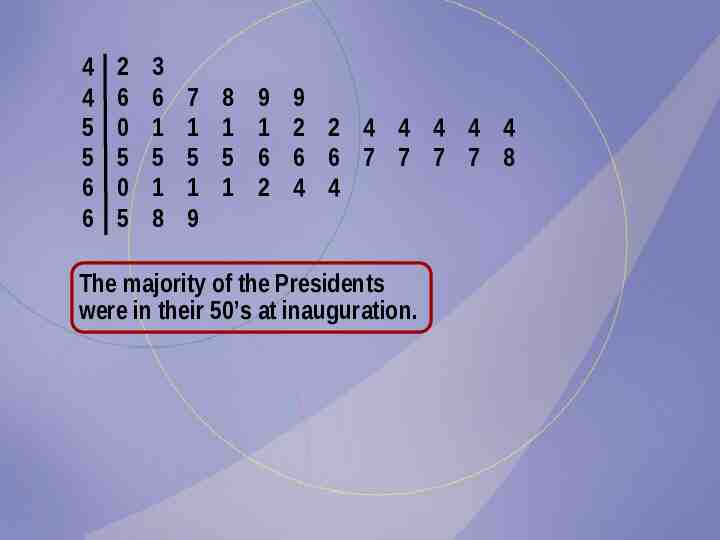
4 4 5 5 6 6 2 6 0 5 0 5 3 6 1 5 1 8 7 1 5 1 9 8 1 5 1 9 1 6 2 9 2 2 4 4 4 4 4 6 6 7 7 7 7 8 4 4 The majority of the Presidents were in their 50’s at inauguration.