EECS 122: Introduction to Computer Networks Performance Modeling

32 Slides252.50 KB
EECS 122: Introduction to Computer Networks Performance Modeling Computer Science Division Department of Electrical Engineering and Computer Sciences University of California, Berkeley Berkeley, CA 94720-1776 Katz, Stoica F04
Outline Motivations Timing diagrams Metrics Evaluation techniques Katz, Stoica F04 2
Motivations Understanding network behavior Improving protocols Verifying correctness of implementation Detecting faults Monitor service level agreements Choosing provides Billing Katz, Stoica F04 3
Outline Motivations Timing diagrams Metrics Evaluation techniques Katz, Stoica F04 4
Timing Diagrams Sending one packet Queueing Switching - Store and forward - Cut-through Fluid view Katz, Stoica F04 5
Definitions Link bandwidth (capacity): maximum rate (in bps) at which the sender can send data along the link Propagation delay: time it takes the signal to travel from source to destination Packet transmission time: time it takes the sender to transmit all bits of the packet Queuing delay: time the packet need to wait before being transmitted because the queue was not empty when it arrived Processing Time: time it takes a router/switch to process the packet header, manage memory, etc Katz, Stoica F04 6
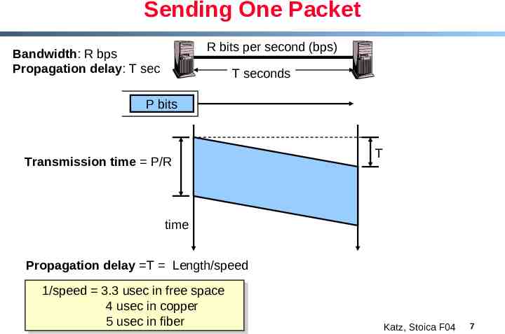
Sending One Packet R bits per second (bps) Bandwidth: R bps Propagation delay: T sec T seconds P bits Transmission time P/R T time Propagation delay T Length/speed 1/speed 3.3 usec in free space 4 usec in copper 5 usec in fiber Katz, Stoica F04 7
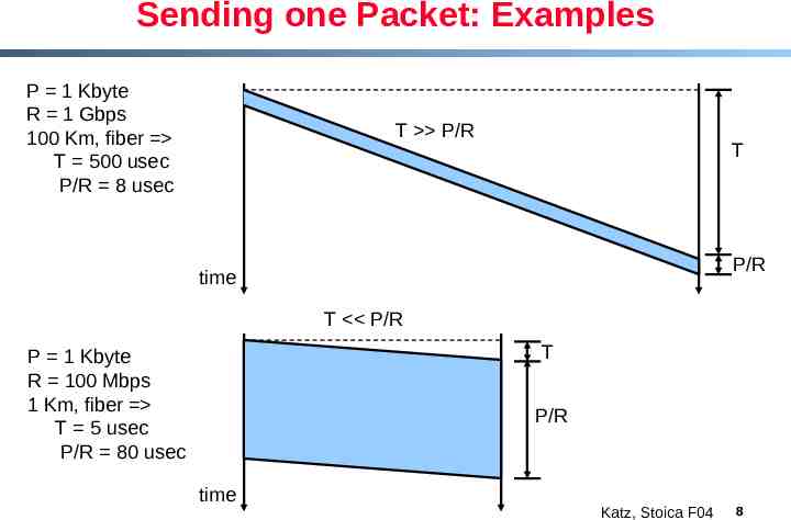
Sending one Packet: Examples P 1 Kbyte R 1 Gbps 100 Km, fiber T 500 usec P/R 8 usec T P/R T P/R time T P/R T P 1 Kbyte R 100 Mbps 1 Km, fiber T 5 usec P/R 80 usec P/R time Katz, Stoica F04 8
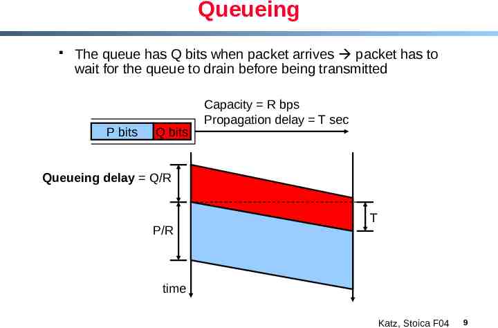
Queueing The queue has Q bits when packet arrives packet has to wait for the queue to drain before being transmitted P bits Q bits Capacity R bps Propagation delay T sec Queueing delay Q/R P/R T time Katz, Stoica F04 9
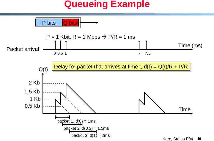
Queueing Example P bits Q bits P 1 Kbit; R 1 Mbps P/R 1 ms Packet arrival Q(t) Time (ms) 0 0.5 1 7 7.5 Delay Delay for for packet packet that that arrives arrives at at time time t,t, d(t) d(t) Q(t)/R Q(t)/R P/R P/R 2 Kb 1.5 Kb 1 Kb 0.5 Kb Time packet 1, d(0) 1ms packet 2, d(0.5) 1.5ms packet 3, d(1) 2ms Katz, Stoica F04 10
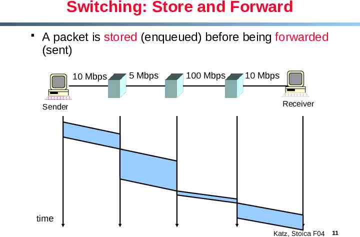
Switching: Store and Forward A packet is stored (enqueued) before being forwarded (sent) 10 Mbps Sender 5 Mbps 100 Mbps 10 Mbps Receiver time Katz, Stoica F04 11
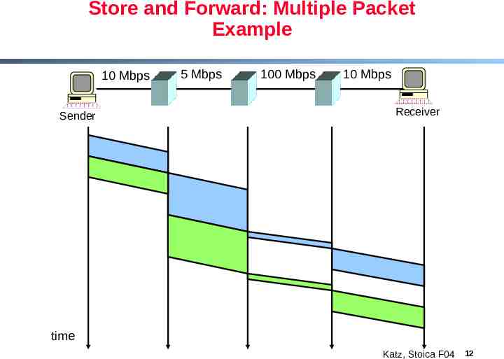
Store and Forward: Multiple Packet Example 10 Mbps Sender 5 Mbps 100 Mbps 10 Mbps Receiver time Katz, Stoica F04 12
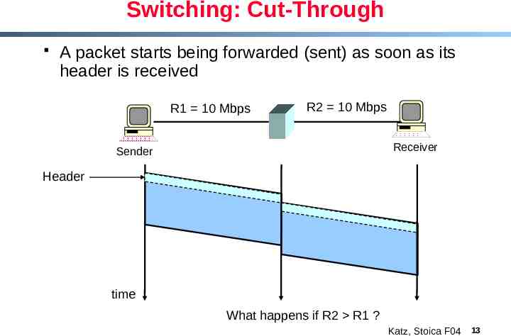
Switching: Cut-Through A packet starts being forwarded (sent) as soon as its header is received R1 10 Mbps R2 10 Mbps Receiver Sender Header time What happens if R2 R1 ? Katz, Stoica F04 13
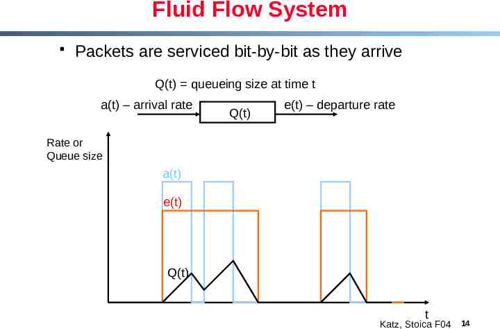
Fluid Flow System Packets are serviced bit-by-bit as they arrive Q(t) queueing size at time t a(t) – arrival rate Q(t) e(t) – departure rate Rate or Queue size a(t) e(t) Q(t) t Katz, Stoica F04 14
Outline Motivations Timing diagrams Metrics Throughput Delay Evaluation techniques Katz, Stoica F04 15
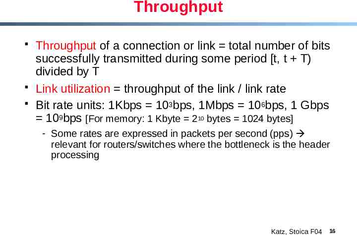
Throughput Throughput of a connection or link total number of bits successfully transmitted during some period [t, t T) divided by T Link utilization throughput of the link / link rate Bit rate units: 1Kbps 103bps, 1Mbps 106bps, 1 Gbps 109bps [For memory: 1 Kbyte 210 bytes 1024 bytes] - Some rates are expressed in packets per second (pps) relevant for routers/switches where the bottleneck is the header processing Katz, Stoica F04 16
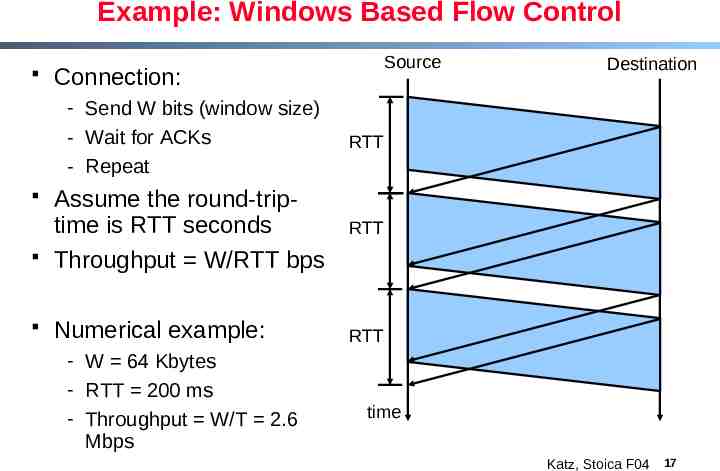
Example: Windows Based Flow Control Connection: Source - Send W bits (window size) - Wait for ACKs - Repeat RTT RTT Assume the round-triptime is RTT seconds Throughput W/RTT bps Numerical example: RTT - W 64 Kbytes - RTT 200 ms - Throughput W/T 2.6 Mbps Destination time Katz, Stoica F04 17
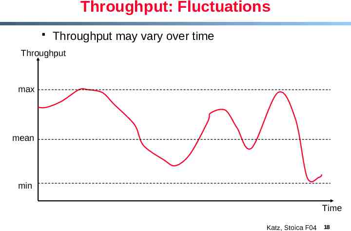
Throughput: Fluctuations Throughput may vary over time Throughput max mean min Time Katz, Stoica F04 18
Delay Delay (Latency) of bit (packet, file) from A to B - The time required for bit (packet, file) to go from A to B Jitter - Variability in delay Round-Trip Time (RTT) - Two-way delay from sender to receiver and back Bandwidth-Delay product - Product of bandwidth and delay “storage” capacity of network Katz, Stoica F04 19
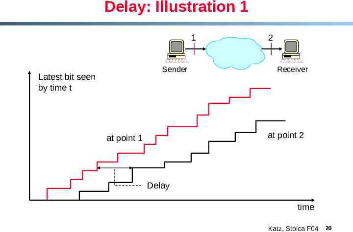
Delay: Illustration 1 1 Sender Latest bit seen by time t 2 Receiver at point 2 at point 1 Delay time Katz, Stoica F04 20
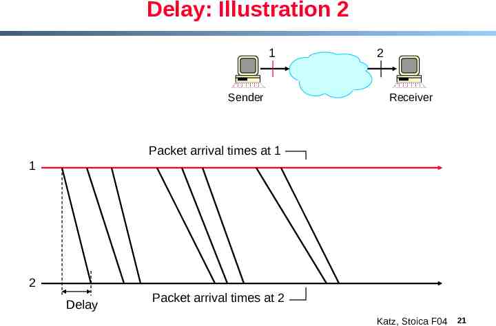
Delay: Illustration 2 1 Sender 2 Receiver Packet arrival times at 1 1 2 Delay Packet arrival times at 2 Katz, Stoica F04 21
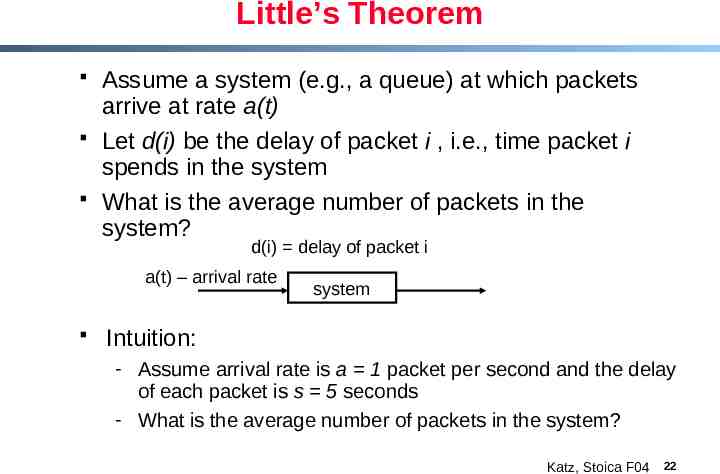
Little’s Theorem Assume a system (e.g., a queue) at which packets arrive at rate a(t) Let d(i) be the delay of packet i , i.e., time packet i spends in the system What is the average number of packets in the system? d(i) delay of packet i a(t) – arrival rate system Intuition: - Assume arrival rate is a 1 packet per second and the delay of each packet is s 5 seconds - What is the average number of packets in the system? Katz, Stoica F04 22
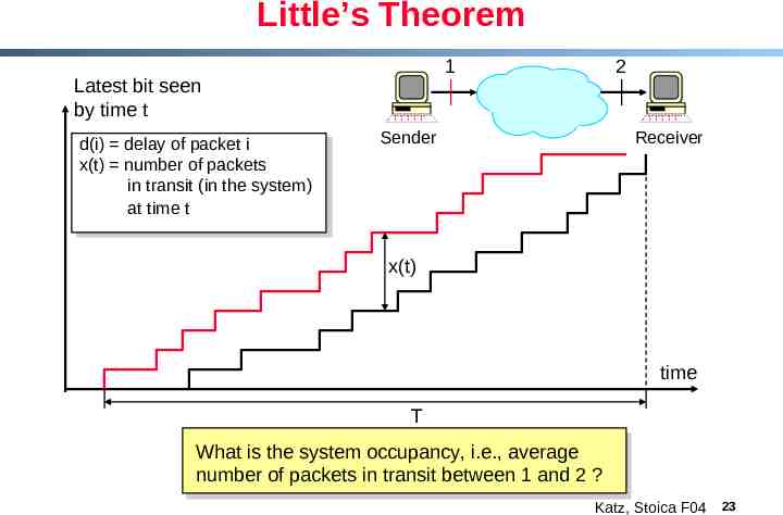
Little’s Theorem 1 Latest bit seen by time t d(i) delay of packet i x(t) number of packets in transit (in the system) at time t 2 Sender Receiver x(t) time T What is the system occupancy, i.e., average number of packets in transit between 1 and 2 ? Katz, Stoica F04 23
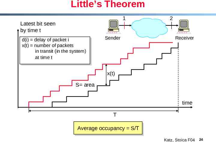
Little’s Theorem 1 Latest bit seen by time t d(i) delay of packet i x(t) number of packets in transit (in the system) at time t Sender 2 Receiver x(t) S area time T Average occupancy S/T Katz, Stoica F04 24
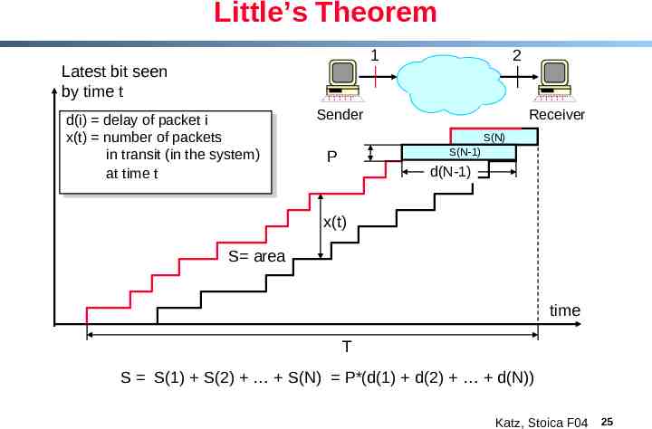
Little’s Theorem 1 Latest bit seen by time t d(i) delay of packet i x(t) number of packets in transit (in the system) at time t 2 Sender Receiver S(N) S(N-1) P d(N-1) x(t) S area time T S S(1) S(2) S(N) P*(d(1) d(2) d(N)) Katz, Stoica F04 25
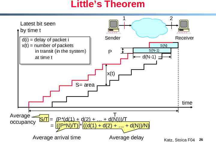
Little’s Theorem 1 Latest bit seen by time t d(i) delay of packet i x(t) number of packets in transit (in the system) at time t 2 Sender Receiver S(N) P S(N-1) d(N-1) x(t) S area time T Average S/T (P*(d(1) d(2) d(N)))/T occupancy ((P*N)/T) * ((d(1) d(2) d(N))/N) Average arrival time Average delay Katz, Stoica F04 26
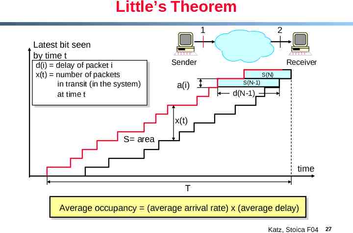
Little’s Theorem 1 Latest bit seen by time t d(i) delay of packet i x(t) number of packets in transit (in the system) at time t 2 Sender Receiver S(N) a(i) S(N-1) d(N-1) x(t) S area time T Average occupancy (average arrival rate) x (average delay) Katz, Stoica F04 27
Outline Motivations Timing diagrams Metrics Evaluation techniques Katz, Stoica F04 28
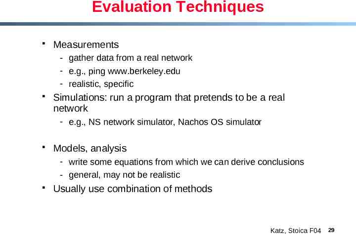
Evaluation Techniques Measurements - gather data from a real network - e.g., ping www.berkeley.edu - realistic, specific Simulations: run a program that pretends to be a real network - e.g., NS network simulator, Nachos OS simulator Models, analysis - write some equations from which we can derive conclusions - general, may not be realistic Usually use combination of methods Katz, Stoica F04 29
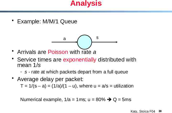
Analysis Example: M/M/1 Queue a s Arrivals are Poisson with rate a Service times are exponentially distributed with mean 1/s - s - rate at which packets depart from a full queue Average delay per packet: T 1/(s – a) (1/a)/(1 – u), where u a/s utilization Numerical example, 1/a 1ms; u 80% Q 5ms Katz, Stoica F04 30
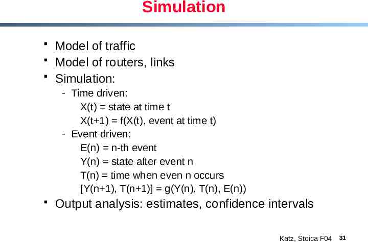
Simulation Model of traffic Model of routers, links Simulation: - Time driven: X(t) state at time t X(t 1) f(X(t), event at time t) - Event driven: E(n) n-th event Y(n) state after event n T(n) time when even n occurs [Y(n 1), T(n 1)] g(Y(n), T(n), E(n)) Output analysis: estimates, confidence intervals Katz, Stoica F04 31
Evaluation: Putting Everything Together Reality Abstraction Plausibility Model Derivation Conclusion Prediction Realism Tractability Hypothesis Usually favor plausibility, tractability over realism - Better to have a few realistic conclusions than none (could not derive) or many conclusions that no one believes (not plausible) Katz, Stoica F04 32