Decomposing, Probing, and Plotting Interactions in Stata


68 Slides2.78 MB
Decomposing, Probing, and Plotting Interactions in Stata https://stats.idre.ucla.edu/stata/seminars/interactions-stata/ 1
Outline Following types of interactions (in linear regression): Continuous by continuous Continuous by categorical Categorical by categorical probe or decompose (defined later) each of these interactions by asking the following research questions: What is the predicted Y given a particular X and W? (predicted value) What is relationship of X on Y at particular values of W? (simple slopes/effects) Is there a difference in the relationship of X on Y for different values of W? (comparing simple slopes) 2
Requirements Basic notions of linear regression Stata installed Dataset loaded into Stata use https://stats.idre.ucla.edu/wp-content/uploads/2020/06/exercise, clear Create value labels label label label label define define values values progl 1 "jog" 2 "swim" 3 "read" genderl 1 "male" 2 "female" prog progl gender genderl Download the complete Stata code here: https://stats.idre.ucla.edu/wp-content/uploads/2020/07/interactions20200724.do 3
Introduction Motivation Main vs. Simple effects (slopes) Predicted Values vs. Slopes 4
Motivation Different types of questions people who spend more time exercising lose more weight (simple regression) more effort people put into their workouts, less time they need to spend exercising (cont x cont) Females and males differ in the amount of weight they lose for the same amount of time (cat x cont) Certain exercise programs may be more effective for females than males (cat x cat) Also, visualize the interaction to help us understand these relationships. 5
Weight Loss Study 900 participants in a year-long study loss: weight loss (continuous), positive weight loss, negative scores weight gain hours: hours spent exercising (continuous) effort: effort during exercise (continuous), 0 minimal physical effort and 50 maximum effort 3 different exercise programs, jogging, swimming and reading (control) prog: exercise program (categorical) jogging 1 swimming 2 reading 3 gender: participant gender (binary) male 1 female 2 6
Definitions decompose: break down the interaction into its lower order components (i.e., predicted means or simple slopes) probe: hypothesis testing to assess the statistical significance of simple slopes and simple slope differences (i.e., interactions) plot: visually display the interaction in the form of simple slopes such as values of the dependent variable are on the y-axis, values of the predictor is on the x-axis, and the moderator separates the lines or bar graphs Elements in the regression model DV: dependent variable (Y), the outcome of your study (e.g., weight loss) IV: independent variable (X), the predictor of your outcome (e.g., time exercising) MV: moderating variable (W) or moderator, a predictor that changes the relationship of the IV on the DV (e.g, effort) coefficient: estimate of the direction and magnitude of the relationship between an IV and DV continuous variable: a variable that can be measured on a continuous scale, e.g., weight, height categorical or binary variable: a variable that takes on discrete values, binary variables take on exactly two values, categorical variables can take on 3 or more values (e.g., gender, ethnicity) Elements of an interaction main effects or slopes: effects or slopes for models that do not involve interaction terms simple slope: when a continuous IV interacts with an MV, its slope at a particular level of an MV simple effect: when a categorical IV interacts with an MV, its effect at a particular level of an MV 7
Regression (Main Effects) Model Outcome Y, two IV’s X and W b0: the intercept, or the predicted outcome when X 0 and W 0. b1: the slope (or main effect) of X; for a one-unit change in X the predicted change in Y b2: the slope (or main effect) of W; for a one-unit change in W the predicted change in Y Only intercept is interpreted at zero Interactions are formed by the product of any two variables. 8
Regression (Interaction) Model b0: the intercept, or the predicted outcome when X 0 and W 0. b1: the simple effect or slope of X, for a one-unit change in X the predicted change in Y at W 0 b2: the simple effect or slope of W, for a one-unit change in W the predicted change in Y at X 0 b3: the interaction of X and W, the change in the slope of X for a one unit increase in W (or vice versa) the intercept fixed at 0 of X and W, each coefficient of an IV interacted with an MV is interpreted at zero of the MV. effect X varies by levels of W identically, effect W varies by levels of X. 9
Regression (Interaction) Model X being the IV and W being the MV, rearrange: coefficient for X is now b1 b3*W X is a function of W Ex. if W 0 slope of X is b1 Ex. if W 1 slope of X is b1 b3 b3 additional increase in the effect or slope of X as W increases by one unit. 10
Predicted Values vs. Slopes regress loss hours We can plug in Hours 2 to get predicted weight loss is 10.02 pounds from 2 hours of exercise 11
Stata’s margins command margins command (Stata 11) post-estimation command to obtain marginal means, predicted values and simple slopes. run a model before running margins (regress) 12
Understanding slopes in regression If delta X 1, then m y2 – y1 7.55 5.08 2.47 13
Slopes in Stata instead of using the at option, we use the option dydx which stands for the slope 14
Plotting a regression slope Sequence 0, 1, 2, 3, 4 Look at the x-axis 15
Quiz #1 True or False? In the margins command, the option dydx is used to estimate predicted values and at is used to estimate simple slopes. Answers are on the last slide. 16
Exercise 1 Refer to the following command What would the plot look like if you replaced the first command with margins, dydx(hours)? Answer is on the next slide. 17
Exercise 1 (solution) 4.32 2.48 0.609 18
Exercise 2 Predict two values of weight loss for Hours 10 and Hours 20 using at, then calculate the slope by hand. How do the results compare with dydx? Answer is on the next slide. 19
Exercise 2 (solution) 20
Continuous by Continuous Model Plotting Simple slopes Differences in predicted values at fixed moderator values 21
Cont x Cont Model Does effort (W) moderate the relationship of Hours (X) on Weight Loss (Y)? Equivalent to: 22
Model Output 𝑊𝑒𝑖𝑔h𝑡𝐿𝑜𝑠𝑠 7.8 9.4 𝐻𝑜𝑢𝑟𝑠 0.08 𝐸𝑓𝑓𝑜𝑟𝑡 0.39 𝐻𝑜𝑢𝑟𝑠 𝐸𝑓𝑓𝑜𝑟𝑡 b0 cons: intercept, or the predicted outcome when Hours 0 and Effort 0. b1 hours: simple slope of Hours, for a one unit change in Hours, the predicted change in weight loss at Effort 0. b2 effort: simple slope of Effort, for a one unit change in Effort the predicted change in weight loss at Hours 0. b3 c.hours#c.effort: interaction of Hours and Effort, change in the slope of Hours for every one unit increase in Effort (or vice versa). 23
Extrapolation (not good) we want to find the predicted weight loss given two hours of exercise and an effort of 30. predicted weight loss is 10.2 pounds if we put in two hours of exercise and an effort level of 30 24
Extrapolation (not good) Predicted weight loss is -10.2 pounds (!!) if we put in two hours of exercise and an effort level of 0. We gain weight from exercising if effort is zero! Nobody in the sample had an effort of zero. (Unlikely scenario) 25
Spotlight analysis (cont x cont) There are an infinite number of (non-extrapolated) simple slopes, use prior research to guide you spotlight analysis: high, medium or low high medium low low medium high 26
Spotlight analysis output Can we marginsplot after this? Slope of Hours is 4.31 at Effort 34.8 (High) 27
Plotting cont x cont interaction order matters x-axis split lines hours spent exercising is only effective for weight loss if we put in more effort (HIIT) 28
Quiz #2 True or False? The command margins, at(hours (0(1)4) effort ( effa eff effb)) tells Stata to plot Hours as the independent variable and Effort as the moderator. 29
Testing simple slopes (cont x cont) Recall simple slopes of hours 2.30 - 4.31 -2.01 30
T- and P- values compared to Interaction From regress From margins Notice sign flip of t-statistic 31
Exercise 3 (Challenge) Recreate the interaction using margins and pwcompare Note: this exercise is exclusive to the slides! Answer is given on the next slide. 32
Answer to Exercise 3 -8.982- (-9.376) 0.394 33
Testing differences in predicted values Instead of testing the difference in slopes (lines), test difference of two predicted values (points) 34
Testing differences in predicted values 35
Testing differences in predicted values 6.88-22.26 -15.38 36
Exercise 4 Estimate the difference in Weight Loss for Low versus High levels of Effort at Hours 0. What is the actual value from Stata? Verify with plot. 37
Answer to Exercise 4 38
Continuous by Categorical Dummy Coding Model Simple slopes Plotting 39
Dummy coding 𝐷 𝑓𝑒𝑚𝑎𝑙𝑒 1if 𝐺𝑒𝑛𝑑𝑒𝑟 𝑓𝑒𝑚𝑎𝑙𝑒 𝐷 𝑓𝑒𝑚𝑎𝑙𝑒 0 if 𝐺𝑒𝑛𝑑𝑒𝑟 𝑚𝑎𝑙𝑒 Note: only dummy codes are required in the regression model e.g., For gender, so only 1 dummy code is required DFEMALE 0 if Gender 1 DFEMALE 1 if Gender 2 40
Dummy codes in regression i. notation makes the lowest value the reference group (Gender 1 or males) 41
Changing the reference group 𝑏 𝐷 𝑊𝑒𝑖𝑔h𝑡𝐿𝑜𝑠𝑠 𝑏 1 2 𝑚𝑎𝑙𝑒 ib2. means make the value of 2 the reference group (Gender 2 or females) 42
Quiz #3 Multiple Choice Refer to the equation What would the equation look like if we made males the reference group? 43
Quiz #4 Multiple Choice Suppose gender 1 codes for Male and gender 2 codes for Female. Write the regression equation for the Stata command regress i.gender 44
Cont x Cat Model Do men and women (MV) differ in the relationship between Hours (IV) and Weight loss? If interacted, the simple slopes are interpreted at 0 of the other variable b0 cons: the intercept, or the predicted weight loss when Hours 0 in the reference group of Gender, which is Dmale 0 or females. b1 hours: simple slope of Hours for the reference group Dmale 0 or females. b2 male: simple effect of Gender or the difference in weight loss between males and females at Hours 0. b3 gender#c.hours: the interaction of Hours and Gender, the difference in the simple slopes of Hours for males versus females. 45
Simple slopes by cat moderator (cont x cat) simple slopes of Hours by gender 46
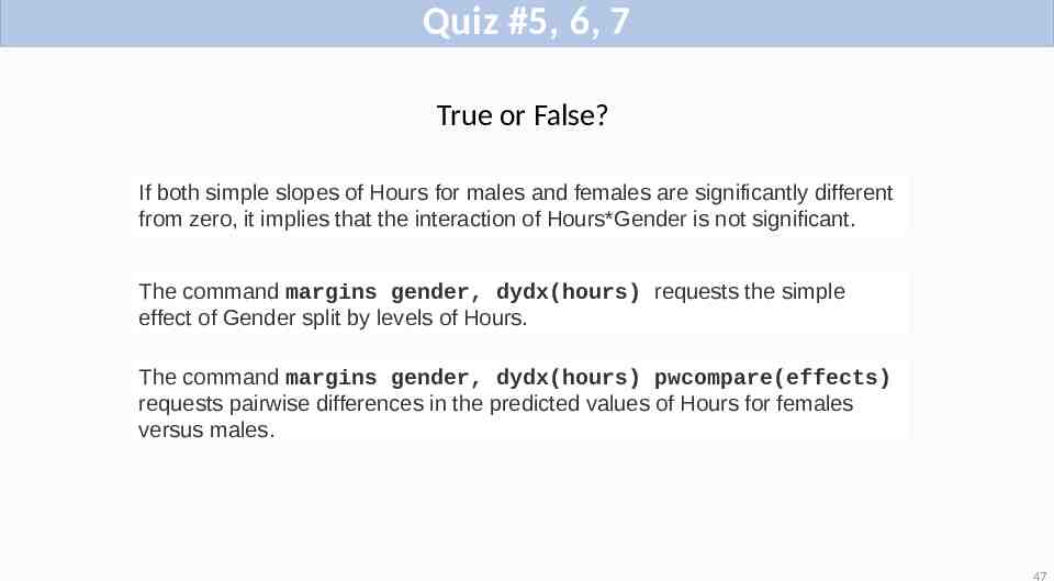
Quiz #5, 6, 7 True or False? If both simple slopes of Hours for males and females are significantly different from zero, it implies that the interaction of Hours*Gender is not significant. The command margins gender, dydx(hours) requests the simple effect of Gender split by levels of Hours. The command margins gender, dydx(hours) pwcompare(effects) requests pairwise differences in the predicted values of Hours for females versus males. 47
Plotting cont x cat interaction 48
Quiz #8, 9 True or False? Looking at the plot in the previous slide, since Hours is on the x-axis it is the IV and Gender separates the lines so it is the moderator (MV). Multiple Choice Refer to the command margins gender, at(hours (0 1 2 3 4)). What is an equivalent way to specify the margins command above, so that we are clear that gender is the moderator? 49
Testing differences in slopes 50
Testing differences in slopes (cont x cat) 3.315-1.591 1.724 51
Compare to regression table 3.315-1.591 1.724 Why are the signs flipped? 52
Categorical by Categorical Model Simple effects Plotting 53
Dummy coding (2 categories) 𝐷𝑚𝑎𝑙𝑒 1 if 𝐺𝑒𝑛𝑑𝑒𝑟 𝑚𝑎𝑙𝑒 𝐷𝑚𝑎𝑙𝑒 0 if 𝐺𝑒𝑛𝑑𝑒𝑟 𝑓𝑒𝑚𝑎𝑙𝑒 Note: only dummy codes are required in the regression model e.g., For gender, so only 1 dummy code is required ib2.gender DMALE 0 if Gender 2 DMALE 1 if Gender 1 54
Dummy Coding (3 categories) Does type of exercise (W) moderate the gender effect (X)? do males and females lose weight differently depending on the type of exercise 𝐷𝑚𝑎𝑙𝑒 1 if 𝐺𝑒𝑛𝑑𝑒𝑟 𝑚𝑎𝑙𝑒 𝐷𝑚𝑎𝑙𝑒 0 if 𝐺𝑒𝑛𝑑𝑒𝑟 𝑓𝑒𝑚𝑎𝑙𝑒 𝐷 𝑗𝑜𝑔 1 , 𝐷𝑠𝑤𝑖𝑚 0if 𝑃𝑟𝑜𝑔 𝑗𝑜𝑔 𝐷 𝑗𝑜𝑔 0 , 𝐷 𝑠𝑤𝑖𝑚 1if 𝑃𝑟𝑜𝑔 𝑠𝑤𝑖𝑚 only k-1 needed, k 2 only k-1 needed, k 3 𝐷 𝑗𝑜𝑔 0 , 𝐷 𝑠𝑤𝑖𝑚 0 if 𝑃𝑟𝑜𝑔 𝑟𝑒𝑎𝑑 𝐷 𝑗𝑜𝑔 1 , 𝐷𝑠𝑤𝑖𝑚 1 if 𝑃𝑟𝑜𝑔 ? 55
Value labels Recall Stata i. notation Gender 2 reference Female Verify DMALE Prog 3 reference Reading DJOG, DSWIM 56
Quiz #10 True or False When we specify ib2.prog Stata internally creates two dummy variables for Categories 1 and 3 57
Cat x Cat Model Equivalent to: must have i. notation or Stata will think the variable is continuous 58
Model Interpretation (Cat x Cat) b0 cons: intercept or the predicted weight loss when Dmale 0 and Djog 0,Dswim 0 (i.e., reading females) b1 male: simple effect of males for Djog 0,Dswim 0 (i.e., male – female weight loss in reading) b2 jog: simple effect of jogging when Dmale 0 (i.e., difference in weight loss between jogging vs reading for females) b3 swim: simple effect of swimming when Dmale 0 (i.e., difference in weight loss between swimming vs reading for females) 59
Model Interpretation (Cat x Cat) b4 male#jog: interaction of Dmale and Djog, the male effect (male – female) in jogging vs the male effect in reading. Also, jogging effect (jogging – reading) for males vs the jogging effect for females b5 male#swim: interaction of Dmale and Dswim, the male effect (male – female) in swimming vs male effect in reading. Also, swimming effect (swimming- reading) for males vs the swimming effect for females 60
Interaction as the additional effect male male#jog male effect for jogging b1 male: male effect (male – female) weight loss in reading b4 male#jog: male effect (male – female) in jogging vs the male effect in reading, (i.e., additional effect of jogging) male male#swim male effect for swimming b5 male#swim: male effect (male – female) in swimming vs male effect in reading, (i.e., additional male effect for swimming) 61
Predicted Values (cat x cat) categorical predictors come before comma (not an option) 62
Simple effects not interaction (cat x cat) Even though gender is a categorical variable we must specify dydx after comma Simple male effects reference group, ib2.gender 63
Interaction Difference of Simple Effects (continued) Male effect swimming Male effect reading -6.595 – (-.3354) - 6.259 Difference of simple effects male male#swim male effect for swimming Additional effect 64
Quiz #11, 12 True or False Compare to the Stata command regress loss ib2.gender##ib3.prog. Equivalent syntax is regress loss gender prog ib2.gender#ib3.prog. The interaction male#jog is the male effect for the jogging condition. 65
Plotting cat x cat interaction both categorical so comes before comma x-axis separate lines 66
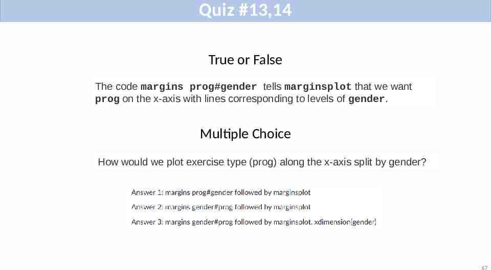
Quiz #13,14 True or False The code margins prog#gender tells marginsplot that we want prog on the x-axis with lines corresponding to levels of gender. Multiple Choice How would we plot exercise type (prog) along the x-axis split by gender? 67
Answers to Quiz Questions 1. F 2. T 3. Answer 2 4. Answer 1 5. F, The test of simple slopes is not the same as the test of the interaction, which tests the difference of simple slopes. 6. F, We are not obtaining the simple effect of Gender but simple slopes of Hours. The statement dydx(hours) indicates the simple slope we are requesting. Since gender is categorical, it comes before the comma which means we want the simple slope of Hours by Gender. 7. F, This is the pairwise difference in the slope of Hours for females versus males. Recall that dydx(hours) obtains simple slopes and at obtains predicted values. 8. T 9. Answer 1 10. T 11. F, Without the i. prefix for the simple effects, Stata treats gender and prog as continuous variables despite the correct ib#. specification in the interaction term. 12. F, The male jogging effect alone does not capture the interaction. The interaction is the difference of simple effects. 13. T 14. Answer 1 68