Multi-Echelon Inventory Management Prof. Larry Snyder Lehigh
38 Slides332.50 KB
Multi-Echelon Inventory Management Prof. Larry Snyder Lehigh University Dept. of Industrial & Systems Engineering OR Roundtable, June 15, 2006
Outline Introduction Overview Network topology Assumptions Deterministic models Stochastic models Decentralized systems Multi-Echelon Inventory – June 15, 2006
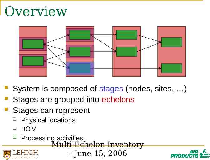
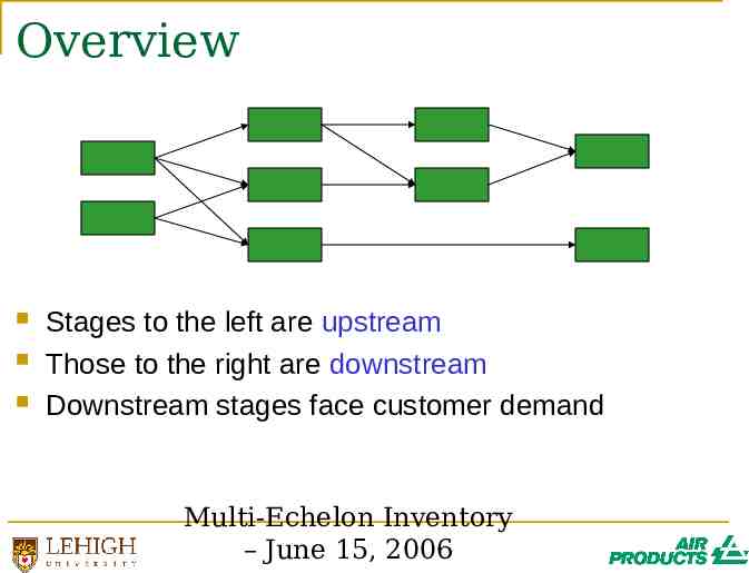
Overview System is composed of stages (nodes, sites, ) Stages are grouped into echelons Stages can represent Physical locations BOM Processing activities Multi-Echelon Inventory – June 15, 2006
Overview Stages to the left are upstream Those to the right are downstream Downstream stages face customer demand Multi-Echelon Inventory – June 15, 2006
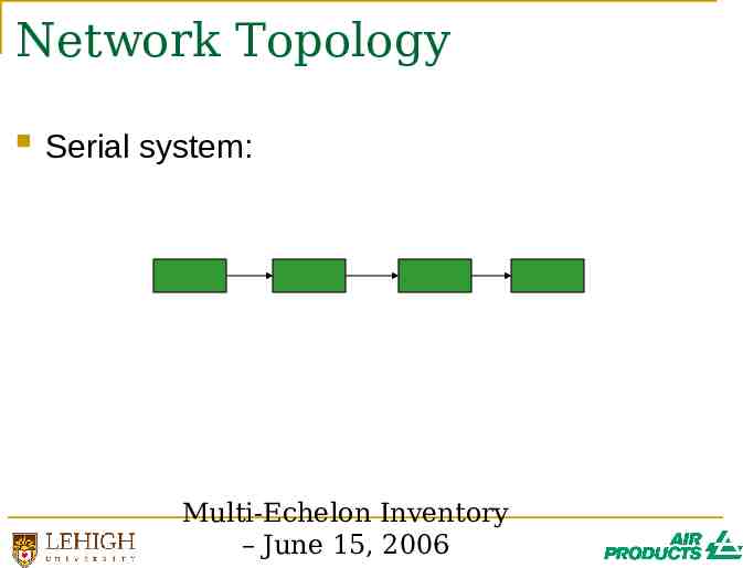
Network Topology Serial system: Multi-Echelon Inventory – June 15, 2006
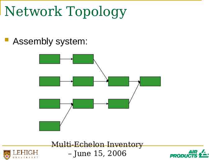
Network Topology Assembly system: Multi-Echelon Inventory – June 15, 2006
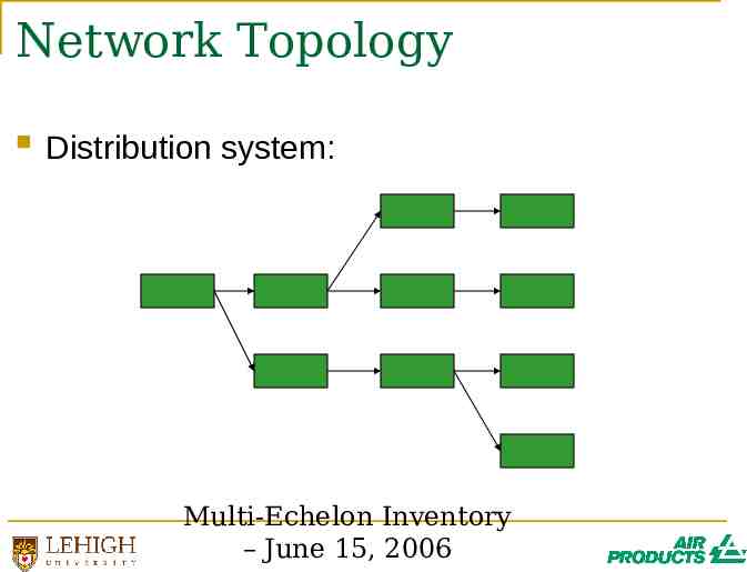
Network Topology Distribution system: Multi-Echelon Inventory – June 15, 2006
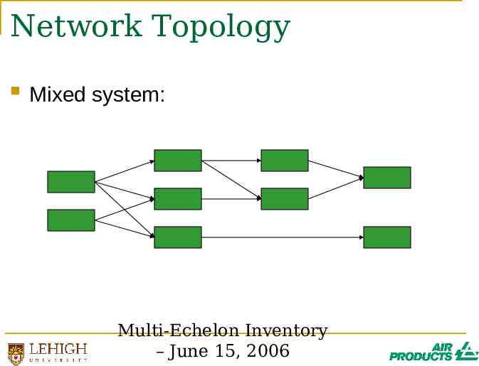
Network Topology Mixed system: Multi-Echelon Inventory – June 15, 2006
Assumptions Periodic review Centralized decision making Period week, month, Can optimize system globally Later, I will talk about decentralized systems Costs Holding cost Fixed order cost Stockout cost (vs. service level) Multi-Echelon Inventory – June 15, 2006
Deterministic Models Suppose everything in the system is deterministic (not random) Demands, lead times, Possible to achieve 100% service If no fixed costs, explode BOM every period If fixed costs are non-negligible, key tradeoff is between fixed and holding costs Multi-echelon version of EOQ MRP systems (optimization component) Multi-Echelon Inventory – June 15, 2006
Outline Introduction Stochastic models Base-stock model Stochastic multi-echelon systems Strategic safety stock placement Supply uncertainty Decentralized systems Multi-Echelon Inventory – June 15, 2006
Stochastic Models Suppose now that demand is stochastic (random) I’ll assume: Still assume supply is deterministic Including lead time, yield, No fixed cost Normally distributed demand: N( , 2) Key tradeoff is between holding and stockout costs Multi-Echelon Inventory – June 15, 2006
The Base-Stock Model Single stage (and echelon) Excess inventory incurs holding cost of h per unit per period Unmet demand is backordered at a cost of p per unit per period Stage follows base-stock policy Each period, “order up to” base-stock level, y aka order-up-to policy Similar to days-of-supply policy: y / DOS Multi-Echelon Inventory – June 15, 2006
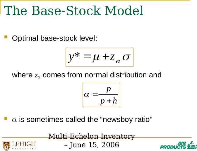
The Base-Stock Model Optimal base-stock level: y* z where z comes from normal distribution and p p h is sometimes called the “newsboy ratio” Multi-Echelon Inventory – June 15, 2006
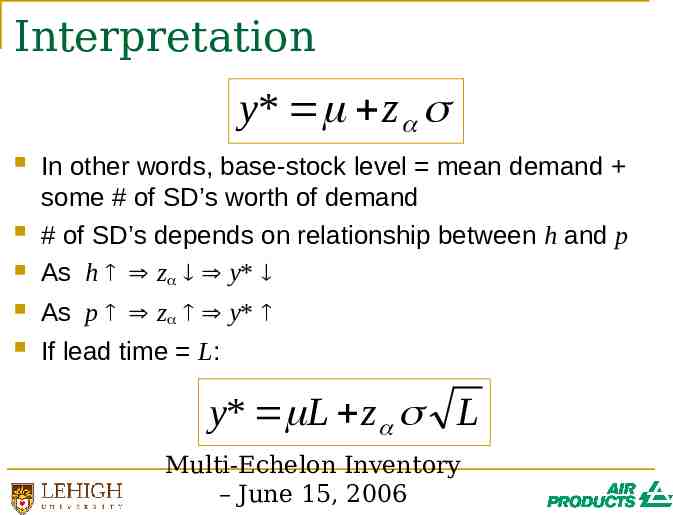
Interpretation y* z In other words, base-stock level mean demand some # of SD’s worth of demand # of SD’s depends on relationship between h and p As h z y* As p z y* If lead time L: y* L z L Multi-Echelon Inventory – June 15, 2006
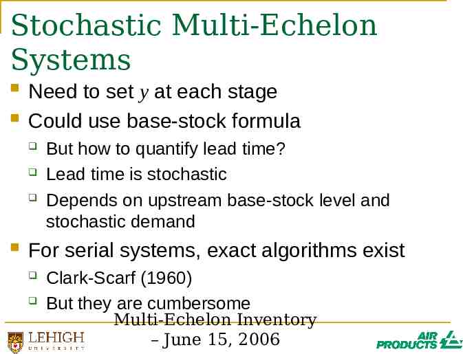
Stochastic Multi-Echelon Systems Need to set y at each stage Could use base-stock formula But how to quantify lead time? Lead time is stochastic Depends on upstream base-stock level and stochastic demand For serial systems, exact algorithms exist Clark-Scarf (1960) But they are cumbersome Multi-Echelon Inventory – June 15, 2006
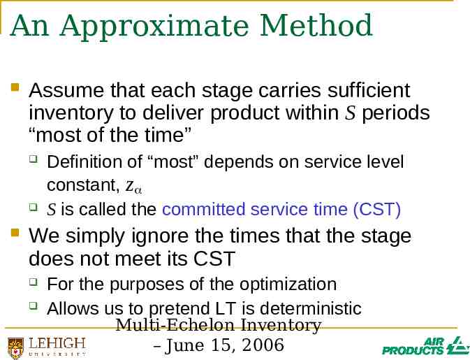
An Approximate Method Assume that each stage carries sufficient inventory to deliver product within S periods “most of the time” Definition of “most” depends on service level constant, z S is called the committed service time (CST) We simply ignore the times that the stage does not meet its CST For the purposes of the optimization Allows us to pretend LT is deterministic Multi-Echelon Inventory – June 15, 2006
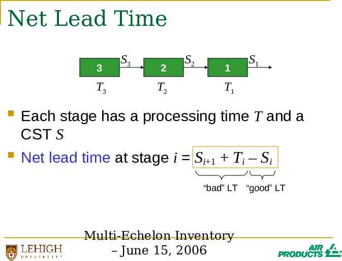
Net Lead Time 3 T3 S3 2 T2 S2 1 S1 T1 Each stage has a processing time T and a CST S Net lead time at stage i Si 1 Ti – Si “bad” LT “good” LT Multi-Echelon Inventory – June 15, 2006
Net Lead Time vs. Inventory Suppose Si Si 1 Ti e.g., inbound CST 4, proc time 2, outbound CST 6 Don’t need to hold any inventory Operate entirely as pull (make-to-order, JIT) system Suppose Si 0 Promise immediate order fulfillment Make-to-stock system Multi-Echelon Inventory – June 15, 2006
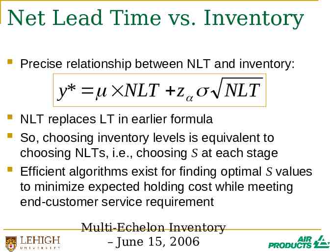
Net Lead Time vs. Inventory Precise relationship between NLT and inventory: y* NLT z NLT NLT replaces LT in earlier formula So, choosing inventory levels is equivalent to choosing NLTs, i.e., choosing S at each stage Efficient algorithms exist for finding optimal S values to minimize expected holding cost while meeting end-customer service requirement Multi-Echelon Inventory – June 15, 2006
Key Insight It is usually optimal for only a few stages to hold inventory Other stages operate as pull systems In a serial system, every stage either: holds zero inventory (and quotes maximum CST) or quotes CST of zero (and holds maximum inventory) Multi-Echelon Inventory – June 15, 2006
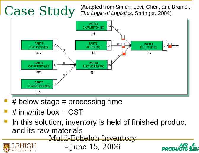
Case Study (Adapted from Simchi-Levi, Chen, and Bramel, The Logic of Logistics, Springer, 2004) PART 2 CHARLESTON ( 7) 14 8 14 PART 5 CHICAGO ( 155) 45 5 45 PART 6 CHARLESTON ( 2) 32 32 8 8 PART 7 CHARLESTON ( 30) PART 3 AUSTIN ( 2) 14 14 PART 4 BALTIMORE ( 220) 6 7 PART 1 DALLAS ( 260) 0 15 55 5 14 14 # below stage processing time # in white box CST In this solution, inventory is held of finished product and its raw materials Multi-Echelon Inventory – June 15, 2006
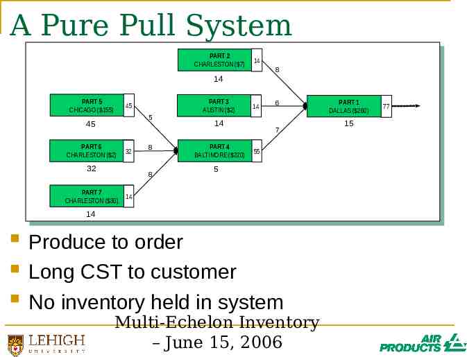
A Pure Pull System PART 2 CHARLESTON ( 7) 14 8 14 PART 5 CHICAGO ( 155) 45 5 45 PART 6 CHARLESTON ( 2) 32 32 8 8 PART 7 CHARLESTON ( 30) PART 3 AUSTIN ( 2) 14 14 PART 4 BALTIMORE ( 220) 6 7 55 5 14 14 Produce to order Long CST to customer No inventory held in system Multi-Echelon Inventory – June 15, 2006 PART 1 DALLAS ( 260) 15 77
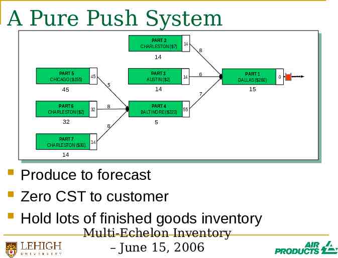
A Pure Push System PART 2 CHARLESTON ( 7) 14 8 14 PART 5 CHICAGO ( 155) 45 5 45 PART 6 CHARLESTON ( 2) 32 32 8 8 PART 7 CHARLESTON ( 30) PART 3 AUSTIN ( 2) 14 14 PART 4 BALTIMORE ( 220) 6 7 PART 1 DALLAS ( 260) 15 55 5 14 14 Produce to forecast Zero CST to customer Hold lots of finished goods inventory Multi-Echelon Inventory – June 15, 2006 0
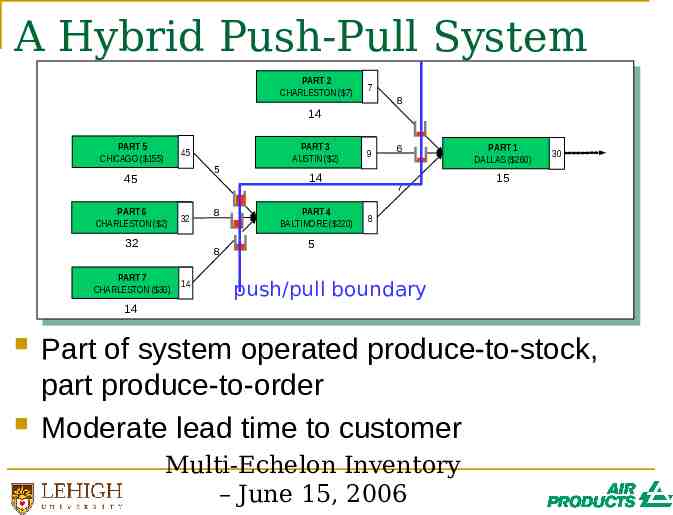
A Hybrid Push-Pull System PART 2 CHARLESTON ( 7) 7 8 14 PART 5 CHICAGO ( 155) 45 5 45 PART 6 CHARLESTON ( 2) 32 32 8 8 PART 7 CHARLESTON ( 30) 14 PART 3 AUSTIN ( 2) 9 14 PART 4 BALTIMORE ( 220) 6 7 PART 1 DALLAS ( 260) 30 15 8 5 push/pull boundary 14 Part of system operated produce-to-stock, part produce-to-order Moderate lead time to customer Multi-Echelon Inventory – June 15, 2006
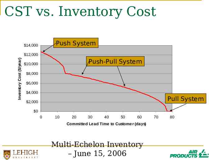
CST vs. Inventory Cost Push System 14,000 Inventory Cost ( /year) 12,000 Push-Pull System 10,000 8,000 6,000 4,000 Pull System 2,000 0 0 10 20 30 40 50 60 Committed Lead Time to Customer (days) Multi-Echelon Inventory – June 15, 2006 70 80
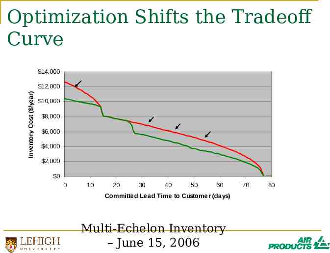
Optimization Shifts the Tradeoff Curve 14,000 Inventory Cost ( /year) 12,000 10,000 8,000 6,000 4,000 2,000 0 0 10 20 30 40 50 60 Committed Lead Time to Customer (days) Multi-Echelon Inventory – June 15, 2006 70 80
Supply Uncertainty Types of supply uncertainty: Strategies for dealing with demand and supply uncertainty are similar Lead-time uncertainty Yield uncertainty Disruptions Safety stock inventory Dual sourcing Improved forecasts But the two are not the same Multi-Echelon Inventory – June 15, 2006
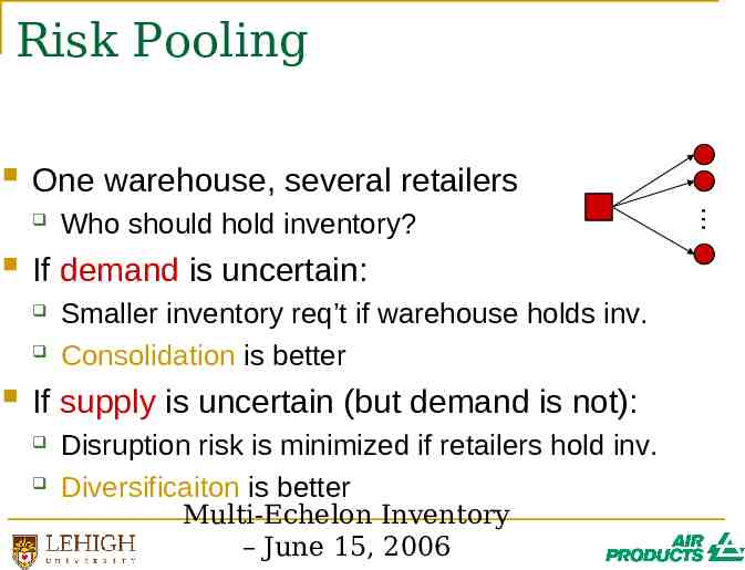
Risk Pooling One warehouse, several retailers If demand is uncertain: Who should hold inventory? Smaller inventory req’t if warehouse holds inv. Consolidation is better If supply is uncertain (but demand is not): Disruption risk is minimized if retailers hold inv. Diversificaiton is better Multi-Echelon Inventory – June 15, 2006
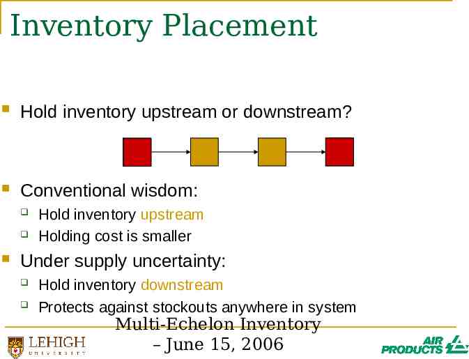
Inventory Placement Hold inventory upstream or downstream? Conventional wisdom: Hold inventory upstream Holding cost is smaller Under supply uncertainty: Hold inventory downstream Protects against stockouts anywhere in system Multi-Echelon Inventory – June 15, 2006
Outline Introduction Stochastic models Decentralized systems Suboptimality Contracting The bullwhip effect Multi-Echelon Inventory – June 15, 2006
Decentralized Systems So far, we have assumed the system is centralized Can optimize at all stages globally One stage may incur higher costs to benefit the system as a whole What if each stage acts independently to minimize its own cost / maximize its own profit? Multi-Echelon Inventory – June 15, 2006
Suboptimality Optimizing locally is likely to result in some degree of suboptimality Example: upstream stages want to operate make-to-order Results in too much inventory downstream Another example: Wholesaler chooses wholesale price Retailer chooses order quantity Optimizing independently, the two parties will always leave money on the table Multi-Echelon Inventory – June 15, 2006
Contracting One solution is for the parties to impose a contracting mechanism Splits the costs / profits / risks / rewards Still allows each party to act in its own best interest If structured correctly, system achieves optimal cost / profit, even with parties acting selfishly There is a large body of literature on contracting In practice, idea is commonly used Actual OR models rarely implemented Multi-Echelon Inventory – June 15, 2006
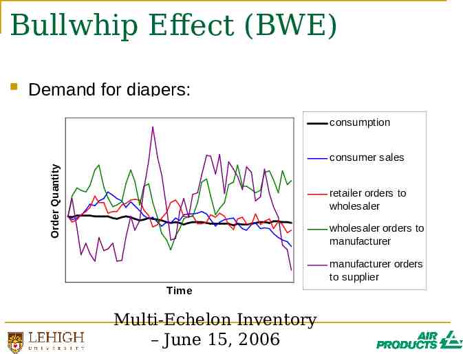
Bullwhip Effect (BWE) Demand for diapers: consumption consumer sales Order Quantity retailer orders to wholesaler wholesaler orders to manufacturer manufacturer orders to supplier Time Multi-Echelon Inventory – June 15, 2006
Irrational Behavior Causes BWE Firms over-react to demand signals Order too much when they perceive an upward demand trend Then back off when they accumulate too much inventory Firms under-weight the supply line Both are irrational behaviors Demonstrated by “beer game” Multi-Echelon Inventory – June 15, 2006
Rational Behavior Causes BWE Famous paper by Hau Lee, et al. (1997) BWE can be cause by rational behavior i.e., by acting in “optimal” ways according to OR inventory models Four causes: Demand forecast updating Batch ordering Rationing game Price variations Multi-Echelon Inventory – June 15, 2006
Questions?