Data Warehouse Tuning


22 Slides134.50 KB
Data Warehouse Tuning
Datawarehouse Tuning Aggregate (strategic) targeting: – Aggregates flow up from a wide selection of data, and then – Targeted decisions flow down Examples: – Riding the wave of clothing fads – Tracking delays for frequent-flyer customers 7 - Datawarehouse 2
Data Warehouse Workload Broad – Aggregate queries over ranges of values, e.g., find the total sales by region and quarter. Deep – Queries that require precise individualized information, e.g., which frequent flyers have been delayed several times in the last month? Dynamic (vs. Static) – Queries that require up-to-date information, e.g. which nodes have the highest traffic now? 7 - Datawarehouse 3
Tuning Knobs Indexes Materialized views Approximation 7 - Datawarehouse 4
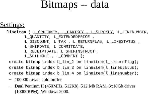
Bitmaps -- data Settings: lineitem ( L ORDERKEY, L PARTKEY , L SUPPKEY, L LINENUMBER, L QUANTITY, L EXTENDEDPRICE , L DISCOUNT, L TAX , L RETURNFLAG, L LINESTATUS , L SHIPDATE, L COMMITDATE, L RECEIPTDATE, L SHIPINSTRUCT , L SHIPMODE , L COMMENT ); create bitmap index b lin 2 on lineitem(l returnflag); create bitmap index b lin 3 on lineitem(l linestatus); create bitmap index b lin 4 on lineitem(l linenumber); – 100000 rows ; cold buffer – Dual Pentium II (450MHz, 512Kb), 512 Mb RAM, 3x18Gb drives (10000RPM), Windows 2000.
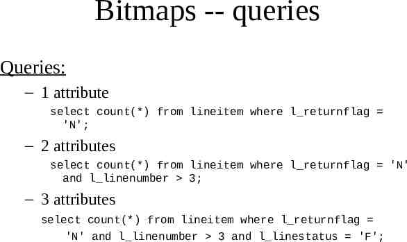
Bitmaps -- queries Queries: – 1 attribute select count(*) from lineitem where l returnflag 'N'; – 2 attributes select count(*) from lineitem where l returnflag 'N' and l linenumber 3; – 3 attributes select count(*) from lineitem where l returnflag 'N' and l linenumber 3 and l linestatus 'F';
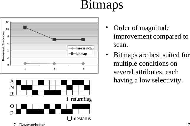
Bitmaps Throughput (Queries/sec) 12 10 8 6 linear scan 4 bitmap 2 0 1 A N R O F 7 - Datawarehouse 2 3 Order of magnitude improvement compared to scan. Bitmaps are best suited for multiple conditions on several attributes, each having a low selectivity. l returnflag l linestatus 7
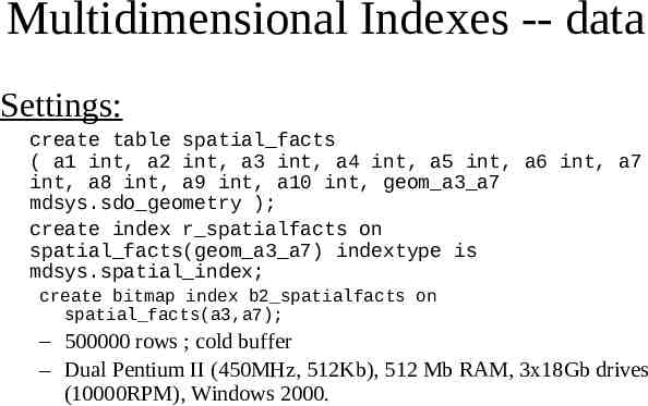
Multidimensional Indexes -- data Settings: create table spatial facts ( a1 int, a2 int, a3 int, a4 int, a5 int, a6 int, a7 int, a8 int, a9 int, a10 int, geom a3 a7 mdsys.sdo geometry ); create index r spatialfacts on spatial facts(geom a3 a7) indextype is mdsys.spatial index; create bitmap index b2 spatialfacts on spatial facts(a3,a7); – 500000 rows ; cold buffer – Dual Pentium II (450MHz, 512Kb), 512 Mb RAM, 3x18Gb drives (10000RPM), Windows 2000.
Multidimensional Indexes -queries Queries: – Point Queries select count(*) from fact where a3 694014 and a7 928878; select count(*) from spatial facts where SDO RELATE(geom a3 a7, MDSYS.SDO GEOMETRY(2001, NULL, MDSYS.SDO POINT TYPE(694014,928878, NULL), NULL, NULL), 'mask equal querytype WINDOW') 'TRUE'; – Range Queries select count(*) from spatial facts where SDO RELATE(geom a3 a7, mdsys.sdo geometry(2003,NULL,NULL, mdsys.sdo elem info array(1,1003,3),mdsys.sdo ordinate array(10,8000 00,1000000,1000000)), 'mask inside querytype WINDOW') 'TRUE'; select count(*) from spatial facts where a3 10 and a3 1000000 and a7 800000 and a7 1000000;
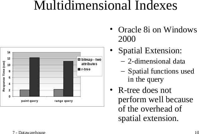
Multidimensional Indexes Oracle 8i on Windows 2000 Spatial Extension: 14 Response Time (sec) 12 bitmap - two attributes 10 r-tree 8 6 4 2 0 point que ry 7 - Datawarehouse ra nge que ry – 2-dimensional data – Spatial functions used in the query R-tree does not perform well because of the overhead of spatial extension. 10
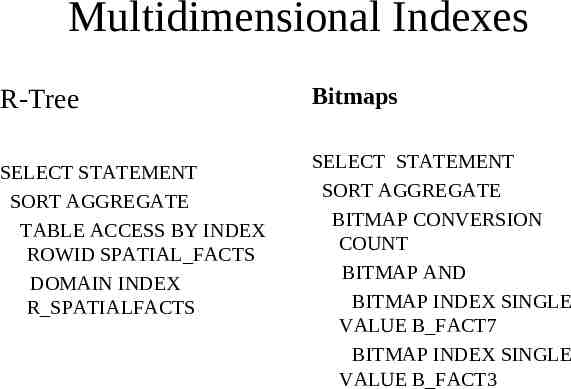
Multidimensional Indexes R-Tree SELECT STATEMENT SORT AGGREGATE TABLE ACCESS BY INDEX ROWID SPATIAL FACTS DOMAIN INDEX R SPATIALFACTS Bitmaps SELECT STATEMENT SORT AGGREGATE BITMAP CONVERSION COUNT BITMAP AND BITMAP INDEX SINGLE VALUE B FACT7 BITMAP INDEX SINGLE VALUE B FACT3
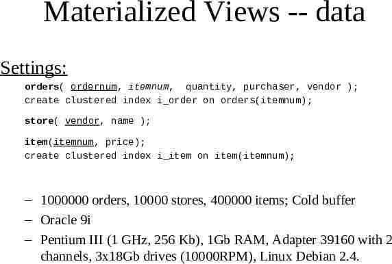
Materialized Views -- data Settings: orders( ordernum, itemnum, quantity, purchaser, vendor ); create clustered index i order on orders(itemnum); store( vendor, name ); item(itemnum, price); create clustered index i item on item(itemnum); – 1000000 orders, 10000 stores, 400000 items; Cold buffer – Oracle 9i – Pentium III (1 GHz, 256 Kb), 1Gb RAM, Adapter 39160 with 2 channels, 3x18Gb drives (10000RPM), Linux Debian 2.4.
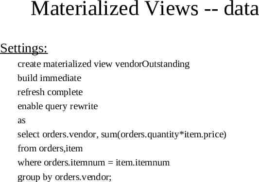
Materialized Views -- data Settings: create materialized view vendorOutstanding build immediate refresh complete enable query rewrite as select orders.vendor, sum(orders.quantity*item.price) from orders,item where orders.itemnum item.itemnum group by orders.vendor;
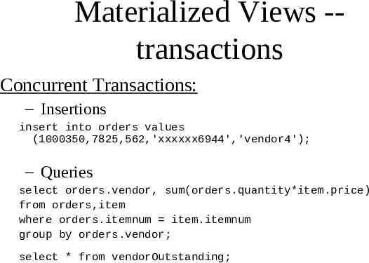
Materialized Views -transactions Concurrent Transactions: – Insertions insert into orders values (1000350,7825,562,'xxxxxx6944','vendor4'); – Queries select orders.vendor, sum(orders.quantity*item.price) from orders,item where orders.itemnum item.itemnum group by orders.vendor; select * from vendorOutstanding;
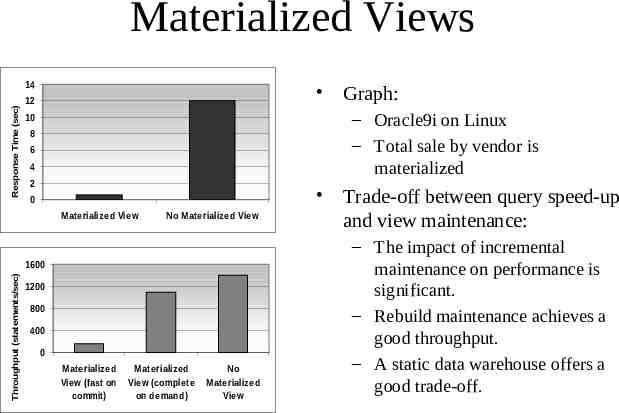
Materialized Views Response Time (sec) 14 Graph: 12 – Oracle9i on Linux – Total sale by vendor is materialized 10 8 6 4 2 0 M aterialized View No Materialized View Throughput (statements/sec) 1600 1200 800 400 0 Materialized View (fast on commit) M aterialized View (complete on demand) No Materialized View Trade-off between query speed-up and view maintenance: – The impact of incremental maintenance on performance is significant. – Rebuild maintenance achieves a good throughput. – A static data warehouse offers a good trade-off.
Materialized View Maintenance Problem when large number of views to maintain. The order in which views are maintained is important: – A view can be computed from an existing view instead of being recomputed from the base relations (total per region can be computed from total per nation). Let the views and base tables be nodes v i Let there be an edge from v 1 to v 2 if it possible to compute the view v 2 from v 1. Associate the cost of computing v 2 from v 1 to this edge. Compute all pairs shortest path where the start nodes are the set of base tables. The result is an acyclic graph A. Take a topological sort of A and let that be the order of view construction.
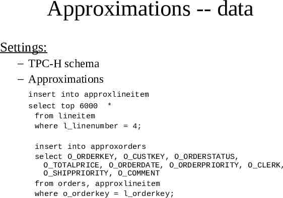
Approximations -- data Settings: – TPC-H schema – Approximations insert into approxlineitem select top 6000 * from lineitem where l linenumber 4; insert into approxorders select O ORDERKEY, O CUSTKEY, O ORDERSTATUS, O TOTALPRICE, O ORDERDATE, O ORDERPRIORITY, O CLERK, O SHIPPRIORITY, O COMMENT from orders, approxlineitem where o orderkey l orderkey;
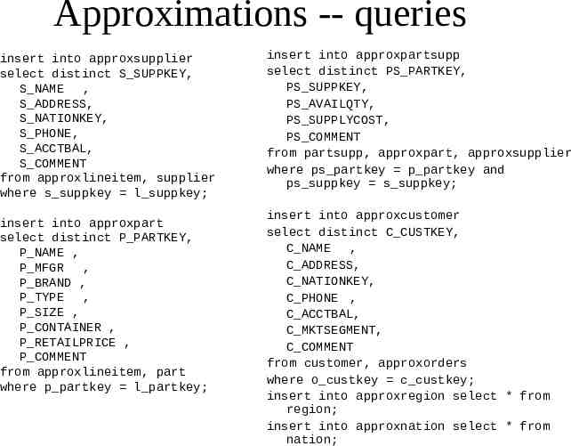
Approximations -- queries insert into approxsupplier select distinct S SUPPKEY, S NAME , S ADDRESS, S NATIONKEY, S PHONE, S ACCTBAL, S COMMENT from approxlineitem, supplier where s suppkey l suppkey; insert into approxpart select distinct P PARTKEY, P NAME , P MFGR , P BRAND , P TYPE , P SIZE , P CONTAINER , P RETAILPRICE , P COMMENT from approxlineitem, part where p partkey l partkey; insert into approxpartsupp select distinct PS PARTKEY, PS SUPPKEY, PS AVAILQTY, PS SUPPLYCOST, PS COMMENT from partsupp, approxpart, approxsupplier where ps partkey p partkey and ps suppkey s suppkey; insert into approxcustomer select distinct C CUSTKEY, C NAME , C ADDRESS, C NATIONKEY, C PHONE , C ACCTBAL, C MKTSEGMENT, C COMMENT from customer, approxorders where o custkey c custkey; insert into approxregion select * from region; insert into approxnation select * from nation;
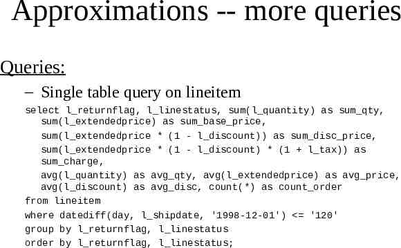
Approximations -- more queries Queries: – Single table query on lineitem select l returnflag, l linestatus, sum(l quantity) as sum qty, sum(l extendedprice) as sum base price, sum(l extendedprice * (1 - l discount)) as sum disc price, sum(l extendedprice * (1 - l discount) * (1 l tax)) as sum charge, avg(l quantity) as avg qty, avg(l extendedprice) as avg price, avg(l discount) as avg disc, count(*) as count order from lineitem where datediff(day, l shipdate, '1998-12-01') '120' group by l returnflag, l linestatus order by l returnflag, l linestatus;
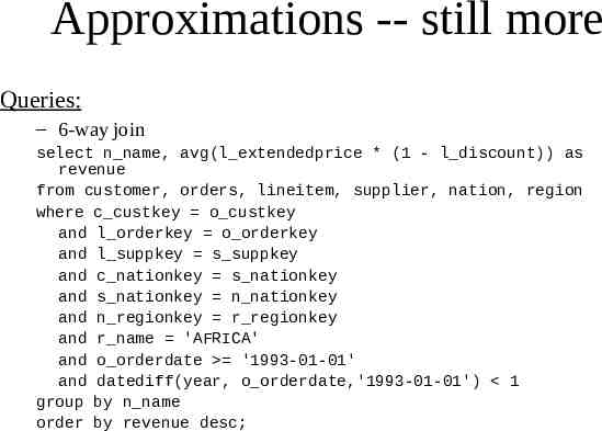
Approximations -- still more Queries: – 6-way join select n name, avg(l extendedprice * (1 - l discount)) as revenue from customer, orders, lineitem, supplier, nation, region where c custkey o custkey and l orderkey o orderkey and l suppkey s suppkey and c nationkey s nationkey and s nationkey n nationkey and n regionkey r regionkey and r name 'AFRICA' and o orderdate '1993-01-01' and datediff(year, o orderdate,'1993-01-01') 1 group by n name order by revenue desc;
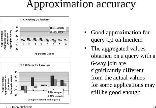
Approximation accuracy Approximated Aggregate Values (% of Base Aggregate Value) T PC-H Query Q1: lineitem 60 1% sample 40 10% sample 20 0 -20 1 2 3 4 5 6 7 -40 Aggregate values TPC-H Query Q5: 6 way join Approximated aggregated values (% of Base Aggregate Value) 60 40 20 0 -20 -40 1 2 3 4 5 1% sample 10% sample Groups returned in the query 7 - Datawarehouse 8 Good approximation for query Q1 on lineitem The aggregated values obtained on a query with a 6-way join are significantly different from the actual values -for some applications may still be good enough. 21
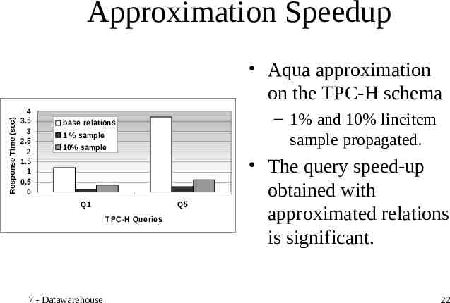
Approximation Speedup Response Time (sec) Aqua approximation on the TPC-H schema 4 3.5 3 2.5 2 1.5 1 0.5 0 – 1% and 10% lineitem sample propagated. base relations 1 % sample 10% sample Q1 Q5 T PC-H Queries 7 - Datawarehouse The query speed-up obtained with approximated relations is significant. 22