Chapter-Six Analysis of fixed income securities

Chapter-Six Analysis of fixed income securities

Introduction Fixed-income securities are those in which their return is fixed, up to some redemption date or indefinitely. The fixed amounts may be stated in money terms or indexed to some measure of the price level. This type of financial investments is presented by two different groups of securities: 1. Long-term debt securities 2. Preferred stocks

Cont’d Long-term debt securities can be described as long-term debt instruments representing the issuer’s contractual obligation. Long term securities have maturity longer than 1 year. The buyer (investor) of these securities is landing money to the issuer, who undertake obligation periodically to pay interest on this loan and repay the principal at a stated maturity date. Long-term debt securities are traded in the capital markets. From the investor’s point of view these securities can be treated as a “safe” asset.

Cont’d But in reality the safety of investment in fixed income securities is strongly related with the default risk of an issuer. The major representatives of long-term debt securities are bonds, but today there are a big variety of different kinds of bonds, which differ not only by the different issuers (governments, municipals, companies, agencies, etc.), but by different schemes of interest payments which is a result of bringing financial innovations to the long-term debt securities market.

Cont’d As demand for borrowing the funds from the capital markets is growing the long-term debt securities today are prevailing in the global markets. And it is really become the challenge for investor to pick long-term debt securities relevant to his/ her investment expectations, including the safety of investment.

Cont’d Preferred stocks are equity security, which has infinitive life and pay dividends. But preferred stock is attributed to the type of fixed-income securities, because the dividend for preferred stock is fixed in amount and known in advance.

Cont’d Though, this security provides for the investor the flow of income very similar to that of the bond. The main difference between preferred stocks and bonds is that for preferred stock the flows are for ever, if the stock is not callable. The preferred stockholders are paid after the debt securities holders but before the common stock holders in terms of priorities in payments of income and in case of liquidation of the company. If the issuer fails to pay the dividend in any year, the unpaid dividends will have to be paid if the issue is cumulative.

Cont’d If preferred stock is issued as noncumulative, dividends for the years with losses do not have to be paid. Usually same rights to vote in general meetings for preferred stockholders are suspended. Because of having the features attributed for both equity and fixed-income securities preferred stocks is known as hybrid security. A most preferred stock is issued as noncumulative and callable. In recent years the preferred stocks with option of convertibility to common stock are proliferating.

6.1. Bond prices and Yields Definition A bond is a long-term contract under which a borrower (the issuer) agrees to make payments of interest and principal, on specific dates, to the holders (creditors) of the bond. It is a fixed income investment in which an investor loans money to an entity (corporate or governmental) that borrows the funds for a defined period of time at a fixed interest rate. Characteristics of Bond .Among the characteristics of bond the following are basic characteristics of bonds. They are typically securities issued by a corporation or governmental body for specified term: bonds become due for payment at maturity, when the par value/ face value of bond are returned to the investors. Bonds usually pay fixed periodic interest installments, called coupon payments. When investor buys bond, he or she becomes a creditor of the issuer. Buyer does not gain any kind of owner ship rights to the issuer, unlike in the case with equity securities

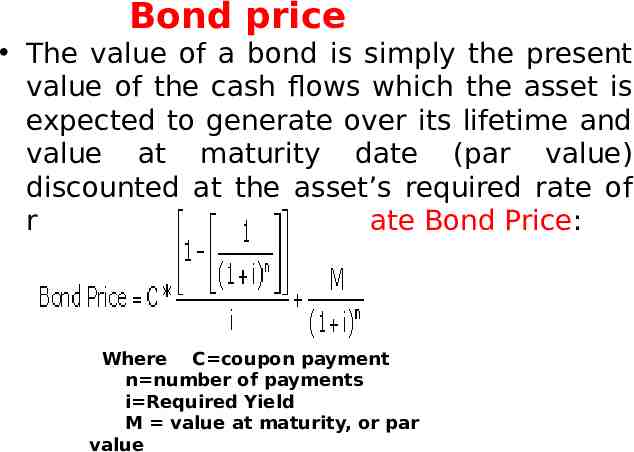
Bond price The value of a bond is simply the present value of the cash flows which the asset is expected to generate over its lifetime and value at maturity date (par value) discounted at the asset’s required rate of return. Formula to calculate Bond Price: Where C coupon payment n number of payments i Required Yield M value at maturity, or par value

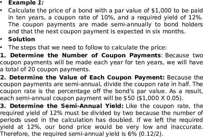
Example 1: Calculate the price of a bond with a par value of 1,000 to be paid in ten years, a coupon rate of 10%, and a required yield of 12%. The coupon payments are made semi-annually to bond holders and that the next coupon payment is expected in six months. Solution The steps that we need to follow to calculate the price: 1. Determine the Number of Coupon Payments: Because two coupon payments will be made each year for ten years, we will have a total of 20 coupon payments. 2. Determine the Value of Each Coupon Payment: Because the coupon payments are semi-annual, divide the coupon rate in half. The coupon rate is the percentage off the bond's par value. As a result, each semi-annual coupon payment will be 50 ( 1,000 X 0.05). 3. Determine the Semi-Annual Yield: Like the coupon rate, the required yield of 12% must be divided by two because the number of periods used in the calculation has doubled. If we left the required yield at 12%, our bond price would be very low and inaccurate. Therefore, the required semi-annual yield is 6% (0.12/2).

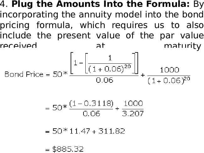
4. Plug the Amounts Into the Formula: By incorporating the annuity model into the bond pricing formula, which requires us to also include the present value of the par value received at maturity Use the formula:

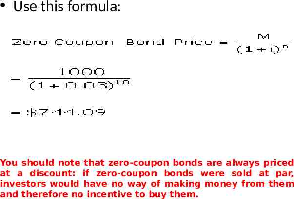
From the above calculation, we have determined that the bond is selling at a discount; the bond price is less than its par value because the required yield of the bond is greater than the coupon rate. The bond must sell at a discount to attract investors, who could find higher interest elsewhere in the prevailing rates. In other words, because investors can make a larger return in the market, they need an extra incentive to invest in the bonds. Zero-Coupon Bond Price What happens when there are no coupon payments? For the zero-coupon bond, there is no coupon payment until maturity. Because of this, the present value of annuity formula is unnecessary. You simply calculate the present value of the par value at maturity. Here's a simple example: Example 2: Let's look at how to calculate the price of

Use this formula: You should note that zero-coupon bonds are always priced at a discount: if zero-coupon bonds were sold at par, investors would have no way of making money from them and therefore no incentive to buy them.

Bond Yields Bond Yield is the return that an investor realize on a bond. It is the function of Bond price and its coupon/ interest payment. There are three widely used measures of the yield 1. Current Yield 2. Yield-to-Maturity 3. Yield- to- Call

1. Current Yield Current yield (CY)- is the simples measure of bond‘s return and has a limited application because it measures only the interest return of the bond. The interpretation of this measure to investor: current yield indicates the amount of current income a bond provides relative to its market price. Use this formula: CY I / Pm Where, I- annual interest of the bond Pm-current market price of the bond

Example: Company Z's issued bonds a 20-year with par value of 1,000 have a price of 970 and annual coupon rate of 9%. Find its current yield. Solution: Annual coupon is 90 ( 1,000 9%) Current market price is 970 so current yield is 90/970 9.28%. 2. Yield- to- Maturity (YTM) is the most important and widely used measure of the bonds returns and key measure in bond valuation process. The percentage rate of return paid on a bond, note, or other fixed income security if the investor buys and holds it to its maturity date. The calculation for YTM is based on the coupon rate, length of time to maturity, and market price. It assumes that coupon interest paid over the life of the bond will be reinvested at the same rate

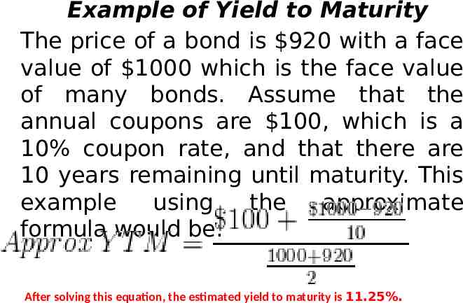
YTM is the fully compounded rate of return earned by an investor in bond over the life of the security, including interest income and price appreciation. Yield-to-maturity can be calculated as an internal rate of return of the bond or the discount rate, which equalizes present value of the future cash flows of the bond to its current market price (value). Use this formula YTM Ct (Pn-P)/n (Pn P)/2 Where, C coupon payment each period(interest Pn - face value of the bond P - current market price of the bond n - number of periods until maturity of the bond; Ct - coupon payment each period(interest), YTM - yield-to-maturity of the bond

Example of Yield to Maturity The price of a bond is 920 with a face value of 1000 which is the face value of many bonds. Assume that the annual coupons are 100, which is a 10% coupon rate, and that there are 10 years remaining until maturity. This example using the approximate formula would be: After solving this equation, the estimated yield to maturity is 11.25%.

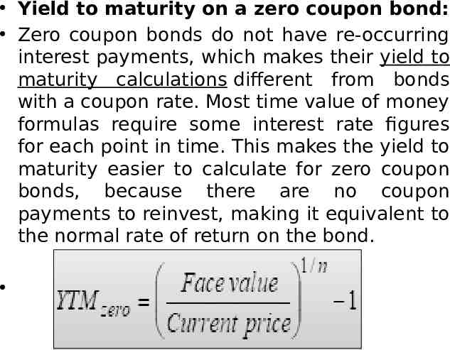
Yield to maturity on a zero coupon bond: Zero coupon bonds do not have re-occurring interest payments, which makes their yield to maturity calculations different from bonds with a coupon rate. Most time value of money formulas require some interest rate figures for each point in time. This makes the yield to maturity easier to calculate for zero coupon bonds, because there are no coupon payments to reinvest, making it equivalent to the normal rate of return on the bond.

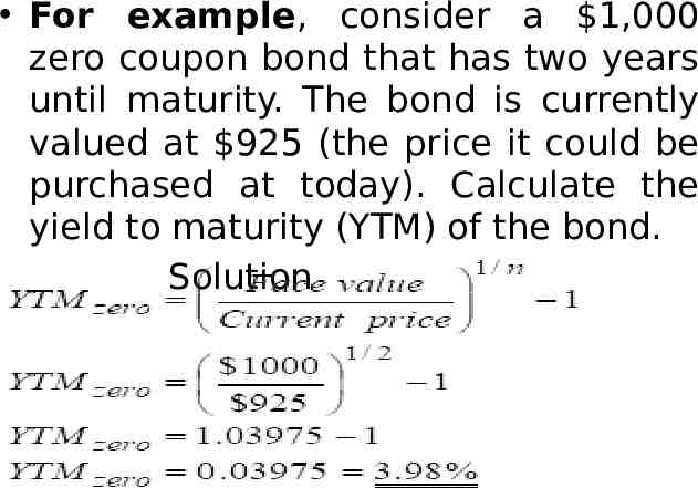
For example, consider a 1,000 zero coupon bond that has two years until maturity. The bond is currently valued at 925 (the price it could be purchased at today). Calculate the yield to maturity (YTM) of the bond. Solution

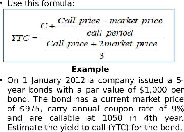
Yield to call As the callable bond gives the issuer the right to retire the bond prematurely, so the issue may or may not remain outstanding to maturity. Thus the YTM may not always be the appropriate measure of value. Instead, the effect of the bond called away prior to maturity must be estimated. For the callable bonds the yield-to-call (YTC) is used. YTC measures the yield on the bond if the issue remains outstanding not to maturity, but rather until its specified call date. YTC can be calculated similar to YTM as an internal rate of return of the bond or the discount rate, which equalizes present value of the future cash flows of the bond to its current market price (value).

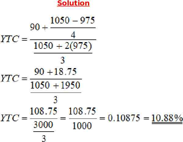
Use this formula: Example On 1 January 2012 a company issued a 5year bonds with a par value of 1,000 per bond. The bond has a current market price of 975, carry annual coupon rate of 9% and are callable at 1050 in 4th year. Estimate the yield to call (YTC) for the bond.

Solution

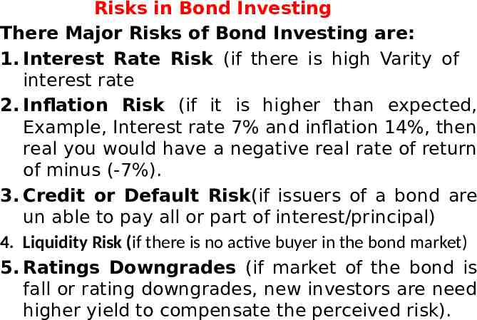
Risks in Bond Investing There Major Risks of Bond Investing are: 1. Interest Rate Risk (if there is high Varity of interest rate 2. Inflation Risk (if it is higher than expected, Example, Interest rate 7% and inflation 14%, then real you would have a negative real rate of return of minus (-7%). 3. Credit or Default Risk(if issuers of a bond are un able to pay all or part of interest/principal) 4. Liquidity Risk (if there is no active buyer in the bond market) 5. Ratings Downgrades (if market of the bond is fall or rating downgrades, new investors are need higher yield to compensate the perceived risk).

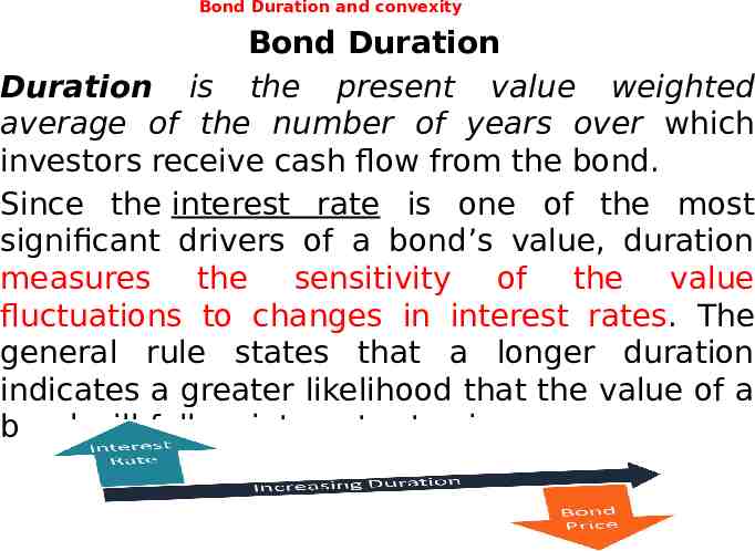
Bond Duration and convexity Bond Duration Duration is the present value weighted average of the number of years over which investors receive cash flow from the bond. Since the interest rate is one of the most significant drivers of a bond’s value, duration measures the sensitivity of the value fluctuations to changes in interest rates. The general rule states that a longer duration indicates a greater likelihood that the value of a bond will fall as interest rates increase.

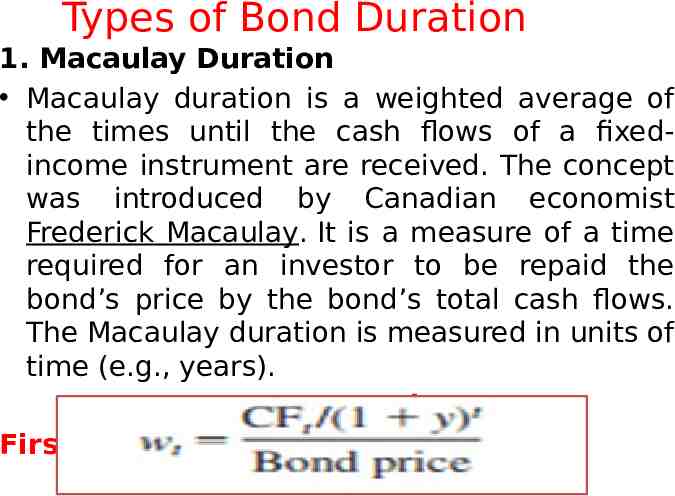
Types of Bond Duration 1. Macaulay Duration Macaulay duration is a weighted average of the times until the cash flows of a fixedincome instrument are received. The concept was introduced by Canadian economist Frederick Macaulay. It is a measure of a time required for an investor to be repaid the bond’s price by the bond’s total cash flows. The Macaulay duration is measured in units of time (e.g., years). Formula First, calculate the weighted average directly as:

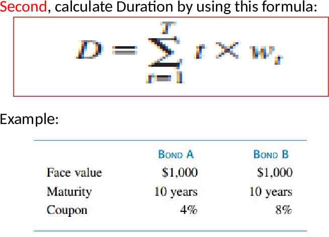
Second, calculate Duration by using this formula: Example:

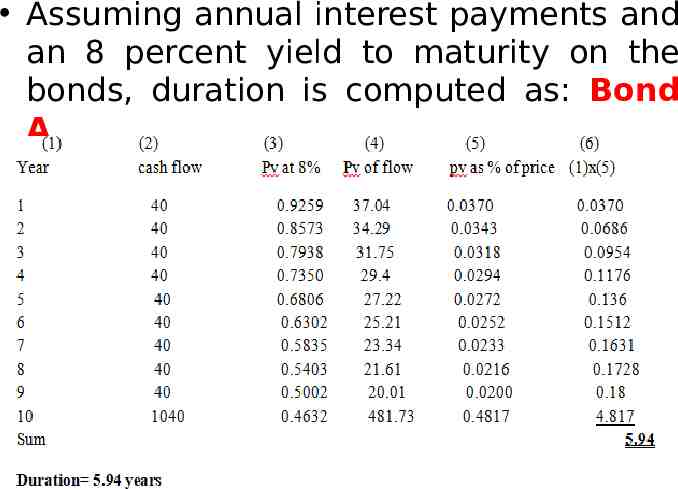
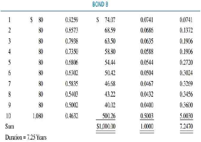
Assuming annual interest payments and an 8 percent yield to maturity on the bonds, duration is computed as: Bond A

Characteristics of Macaulay Duration First, the Macaulay duration of a bond with coupon payments always will be less than its term to maturity because duration gives weight to these interim interest payments. Second, A zero coupon bond or a pure discount bond, such as a Treasury bill, will have duration equal to its term to maturity. If you assume a single payment at maturity, duration will equal term to maturity because the only cash flow comes in the final (maturity) year—that is, you receive 100 percent of cash flows in year n. Third, there is generally a positive relationship between term to maturity and Macaulay duration, but duration increases at a decreasing rate with maturity. Therefore, a bond with longer term to maturity almost always will have a higher duration. Fourth, The shape of the duration-maturity curve depends on the coupon and the yield to maturity. The curve for a zero coupon bond is a straight line, indicating that duration equals term to maturity. In contrast, the curve for a low-coupon bond selling at a deep discount (due to a high YTM) will turn down at long maturities

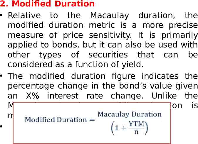
2. Modified Duration Relative to the Macaulay duration, the modified duration metric is a more precise measure of price sensitivity. It is primarily applied to bonds, but it can also be used with other types of securities that can be considered as a function of yield. The modified duration figure indicates the percentage change in the bond’s value given an X% interest rate change. Unlike the Macaulay duration, modified duration is measured in percentages. Formula:

Cont’d Bond Price Change Yield Change Modified Duration Bond Price (calculated as the sum of Present Value of Coupon Payments Present Value of Par Value)

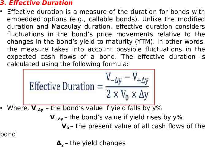
3. Effective Duration Effective duration is a measure of the duration for bonds with embedded options (e.g., callable bonds). Unlike the modified duration and Macaulay duration, effective duration considers fluctuations in the bond’s price movements relative to the changes in the bond’s yield to maturity (YTM). In other words, the measure takes into account possible fluctuations in the expected cash flows of a bond. The effective duration is calculated using the following formula: Where, V–Δy – the bond’s value if yield falls by y% V Δy – the bond’s value if yield rises by y% V0 – the present value of all cash flows of the bond Δy – the yield changes

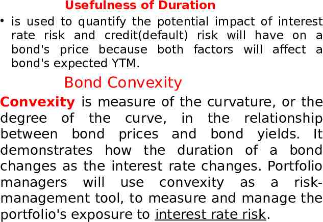
Usefulness of Duration is used to quantify the potential impact of interest rate risk and credit(default) risk will have on a bond's price because both factors will affect a bond's expected YTM. Bond Convexity Convexity is measure of the curvature, or the degree of the curve, in the relationship between bond prices and bond yields. It demonstrates how the duration of a bond changes as the interest rate changes. Portfolio managers will use convexity as a riskmanagement tool, to measure and manage the portfolio's exposure to interest rate risk.

Convexity measures the sensitivity of the bond’s duration to change is yield. Convexity is a good measure for bond price changes with greater fluctuations in the interest rates. Convexity is a risk management tool used to define how risky a bond is as more the convexity of the bond, more is its price sensitivity to interest rate movements. A bond with a higher convexity has larger price change when the interest rate drops than a bond with lower convexity. Hence when two similar bonds are evaluated for investment with similar yield and duration the one with higher convexity is preferred in a stable or falling interest rate scenarios as price change is larger. In a falling interest rate scenario again a higher convexity would be better as the price loss for an increase in interest rates would be smaller.

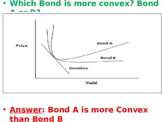
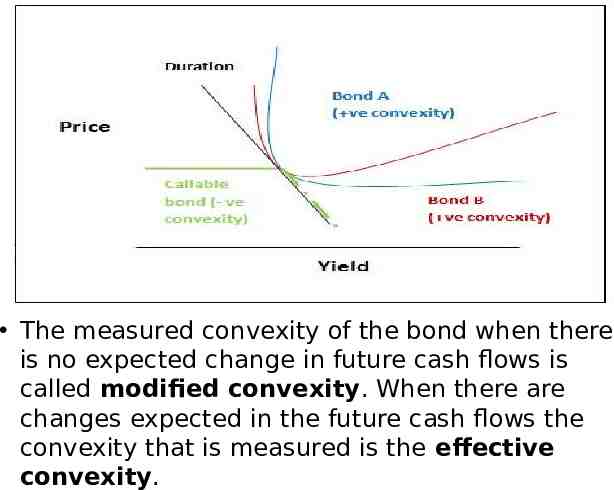
Which Bond is more convex? Bond A or B? Answer: Bond A is more Convex than Bond B

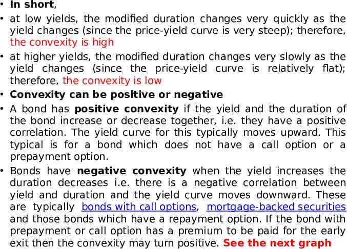
In short, at low yields, the modified duration changes very quickly as the yield changes (since the price-yield curve is very steep); therefore, the convexity is high at higher yields, the modified duration changes very slowly as the yield changes (since the price-yield curve is relatively flat); therefore, the convexity is low Convexity can be positive or negative A bond has positive convexity if the yield and the duration of the bond increase or decrease together, i.e. they have a positive correlation. The yield curve for this typically moves upward. This typical is for a bond which does not have a call option or a prepayment option. Bonds have negative convexity when the yield increases the duration decreases i.e. there is a negative correlation between yield and duration and the yield curve moves downward. These are typically bonds with call options, mortgage-backed securities and those bonds which have a repayment option. If the bond with prepayment or call option has a premium to be paid for the early exit then the convexity may turn positive. See the next graph

The measured convexity of the bond when there is no expected change in future cash flows is called modified convexity. When there are changes expected in the future cash flows the convexity that is measured is the effective convexity.

Major Difference of Bond Duration and Convexity Duration of a bond is the linear relationship between the bond price and interest rates where, as interest rates increase bond price decreases. Simply put, a higher duration implies that the bond price is more sensitive to rate changes. For a small and sudden change in bond yield duration is a good measure of the sensitivity of the bond price. However, for larger changes in yield, the duration measure is not effective as the relationship is non-linear and is a curve. Convexity measures the sensitivity of the bond’s duration to change is yield. Convexity is a good measure for bond price changes with greater fluctuations in the interest rates.

Managing Bond portfolios Two types of strategies investing in bonds: 1. Passive management strategies; 2. Active management strategies 1. Passive bond management strategies A passive investment strategy takes market prices of securities as fairly set.

The main features of the passive management strategies: They are the expression of the little volatile in the investor’s forecasts regarding interest rate and/ or bond price; Have a lower expected return and risk than do active strategies; The small transaction costs. The passive bond management strategies include the following two broad classes of strategies: 1. Indexing strategies. 2. Immunization strategy

The first broad class of passive strategy is an indexing strategy that attempts to replicate the performance of a given bond index. The second broad class of passive strategies is known as immunization techniques; they are used widely by financial institutions such as insurance companies and pension funds, and are designed to shield the overall financial status of the institution from exposure to interest rate fluctuations. A bond-index portfolio will have the same risk-reward profile as the bond market index to which it is tied. In contrast, immunization strategies seek to establish a virtually zero-risk profile, in which interest rate movements have no impact on the value of the firm. It is possible if the bondholder chooses a bond whose duration is equal to his investment horizon. Pure immunization implies that a portfolio is invested for a defined return for a specific period of time regardless of any outside influences, such as changes in interest rates

2. Active Management Strategy Active investment strategy attempts to achieve returns greater than those commensurate with the risk borne. In the context of bond management this style of management can take two forms. Active managers either use interest rate forecasts to predict movements in the entire fixed-income market, or they employ some form of intra market analysis to identify particular sectors of the fixed-income market or particular bonds that are relatively mispriced(identifying over valuate bonds and under valuated bonds). Because interest-rate risk is crucial to formulating both active and passive strategies.

The main classes of active bond management strategies are: 1. The substitution swap: the key to a bond swap strategy is to liquidate the current position and simultaneously purchase another issue with similar characteristics for the sole purpose of improving the portfolio’s return. It is an exchange of one bond for a nearly identical substitute. The substituted bonds should be of essentially equal coupon, maturity, quality, call features, sinking fund provisions, and so on. This swap would be motivated by a belief that the market has temporarily mispriced the two bonds, and that the discrepancy between the prices of the bonds represents a profit

Cont’d 2. The intermarket spread swap is pursued when an investor believes that the yield spread between two sectors of the bond market is temporarily out of line. For example, if the current spread between corporate and government bonds is considered too wide and is expected to narrow, the investor will shift from government bonds into corporate bonds. If the yield spread does in fact narrow, corporates will outperform governments. 3. The rate anticipation swap is pegged to interest rate forecasting. In this case if investors believe that rates will fall, they will swap into bonds of longer duration. Conversely, when rates are expected to rise, they will swap into shorter duration bonds.

End of chapter six!!