CPU Scheduling Chapter 5 1
34 Slides367.50 KB
CPU Scheduling Chapter 5 1
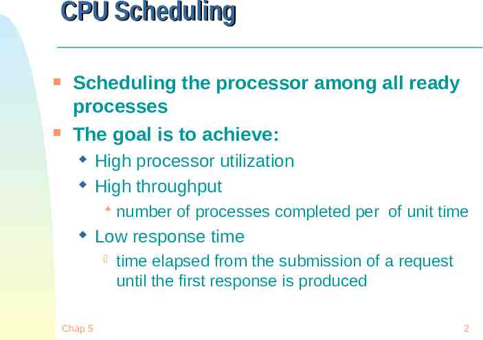
CPU Scheduling Scheduling the processor among all ready processes The goal is to achieve: High processor utilization High throughput Low response time Chap 5 number of processes completed per of unit time time elapsed from the submission of a request until the first response is produced 2
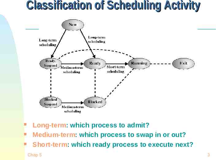
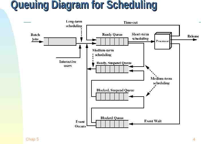
Classification of Scheduling Activity Long-term: which process to admit? Medium-term: which process to swap in or out? Short-term: which ready process to execute next? Chap 5 3
Queuing Diagram for Scheduling Chap 5 4
Long-Term Scheduling Determines which programs are admitted to the system for processing Controls the degree of multiprogramming Attempts to keep a balanced mix of processor-bound and I/O-bound processes Chap 5 CPU usage System performance 5
Medium-Term Scheduling Makes swapping decisions based on the current degree of multiprogramming Controls which remains resident in memory and which jobs must be swapped out to reduce degree of multiprogramming Chap 5 6
Short-Term Scheduling Selects from among ready processes in memory which one is to execute next The selected process is allocated the CPU It is invoked on events that may lead to choose another process for execution: Clock interrupts I/O interrupts Operating system calls and traps Signals Chap 5 7
Characterization of Scheduling Policies The selection function determines which ready process is selected next for execution The decision mode specifies the instants in time the selection function is exercised Nonpreemptive Once a process is in the running state, it will continue until it terminates or blocks for an I/O Preemptive Currently running process may be interrupted and moved to the Ready state by the OS Prevents one process from monopolizing the processor Chap 5 8
Short-Term Scheduler Dispatcher The dispatcher is the module that gives control of the CPU to the process selected by the short-term scheduler The functions of the dispatcher include: Switching context Switching to user mode Jumping to the location in the user program to restart execution The dispatch latency must be minimal Chap 5 9
The CPU-I/O Cycle Processes require alternate use of processor and I/O in a repetitive fashion Each cycle consist of a CPU burst followed by an I/O burst A process terminates on a CPU burst CPU-bound processes have longer CPU bursts than I/O-bound processes Chap 5 10
Short-Tem Scheduling Criteria User-oriented criteria Response Time: Elapsed time between the submission of a request and the receipt of a response Turnaround Time: Elapsed time between the submission of a process to its completion System-oriented criteria Processor utilization Throughput: number of process completed per unit time fairness Chap 5 11
Scheduling Algorithms First-Come, First-Served Scheduling Shortest-Job-First Scheduling Also referred to asShortest Process Next Priority Scheduling Round-Robin Scheduling Multilevel Queue Scheduling Multilevel Feedback Queue Scheduling Chap 5 12
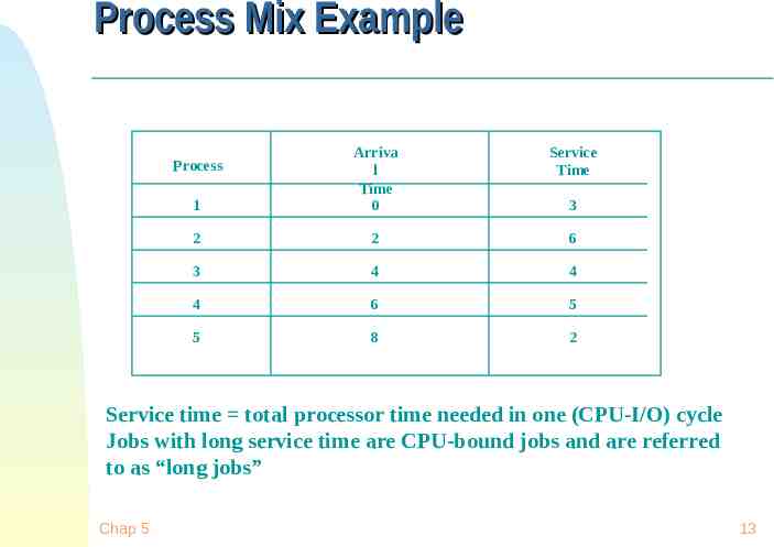
Process Mix Example Service Time 1 Arriva l Time 0 2 2 6 3 4 4 4 6 5 5 8 2 Process 3 Service time total processor time needed in one (CPU-I/O) cycle Jobs with long service time are CPU-bound jobs and are referred to as “long jobs” Chap 5 13
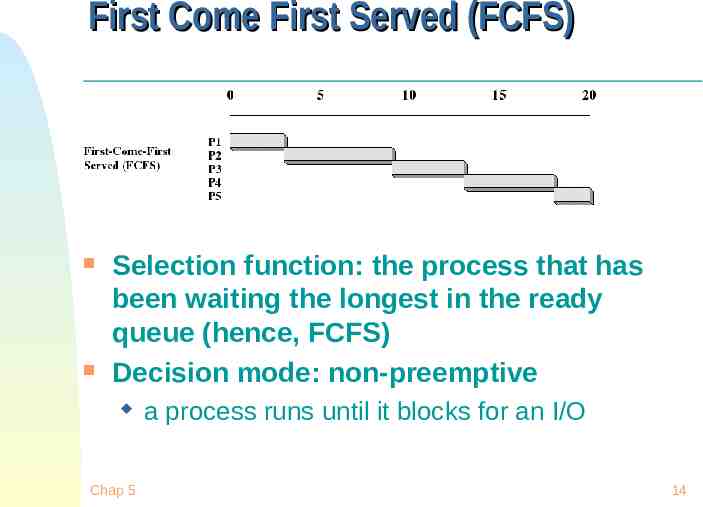
First Come First Served (FCFS) Selection function: the process that has been waiting the longest in the ready queue (hence, FCFS) Decision mode: non-preemptive Chap 5 a process runs until it blocks for an I/O 14
FCFS drawbacks Favors CPU-bound processes A CPU-bound process monopolizes the processor I/O-bound processes have to wait until completion of CPU-bound process Chap 5 I/O-bound processes may have to wait even after their I/Os are completed (poor device utilization) Better I/O device utilization could be achieved if I/O bound processes had higher priority 15
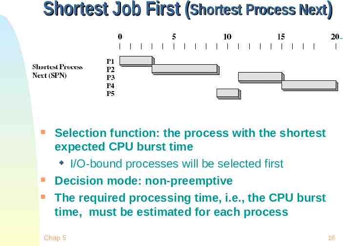
Shortest Job First (Shortest Process Next) Selection function: the process with the shortest expected CPU burst time I/O-bound processes will be selected first Decision mode: non-preemptive The required processing time, i.e., the CPU burst time, must be estimated for each process Chap 5 16
SJF / SPN Critique Possibility of starvation for longer processes Lack of preemption is not suitable in a time sharing environment SJF/SPN implicitly incorporates priorities Chap 5 Shortest jobs are given preferences CPU bound process have lower priority, but a process doing no I/O could still monopolize the CPU if it is the first to enter the system 17
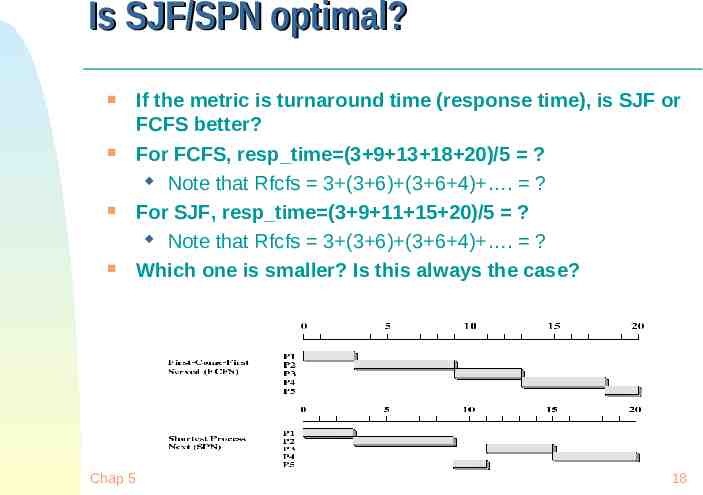
Is SJF/SPN optimal? Chap 5 If the metric is turnaround time (response time), is SJF or FCFS better? For FCFS, resp time (3 9 13 18 20)/5 ? Note that Rfcfs 3 (3 6) (3 6 4) . ? For SJF, resp time (3 9 11 15 20)/5 ? Note that Rfcfs 3 (3 6) (3 6 4) . ? Which one is smaller? Is this always the case? 18
Is SJF/SPN optimal? Take each scheduling discipline, they both choose the same subset of jobs (first k jobs). At some point, each discipline chooses a different job (FCFS chooses k1 SJF chooses k2) Rfcfs nR1 (n-1)R2 (n-k1)Rk1 . (n-k2) Rk2 . Rn Rsjf nR1 (n-1)R2 (n-k2)Rk2 . (n-k1) Rk1 . Rn Which one is smaller? Rfcfs or Rsjf? Chap 5 19
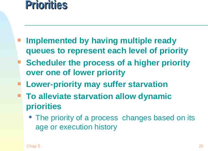
Priorities Implemented by having multiple ready queues to represent each level of priority Scheduler the process of a higher priority over one of lower priority Lower-priority may suffer starvation To alleviate starvation allow dynamic priorities The priority of a process changes based on its age or execution history Chap 5 20
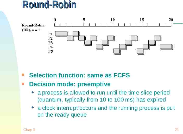
Round-Robin Selection function: same as FCFS Decision mode: preemptive Chap 5 a process is allowed to run until the time slice period (quantum, typically from 10 to 100 ms) has expired a clock interrupt occurs and the running process is put on the ready queue 21
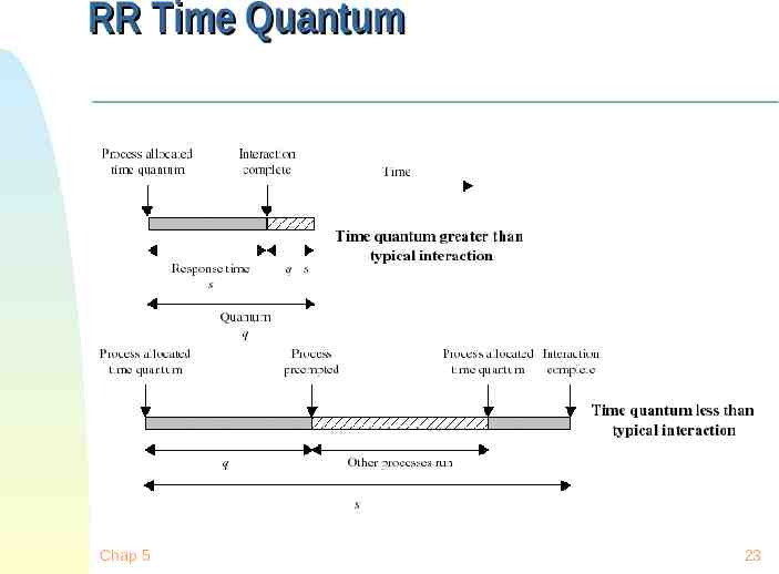
RR Time Quantum Quantum must be substantially larger than the time required to handle the clock interrupt and dispatching Quantum should be larger then the typical interaction but not much larger, to avoid penalizing I/O bound processes Chap 5 22
RR Time Quantum Chap 5 23
Round Robin: critique Still favors CPU-bound processes An I/O bound process uses the CPU for a time less than the time quantum before it is blocked waiting for an I/O A CPU-bound process runs for all its time slice and is put back into the ready queue May unfairly get in front of blocked processes Chap 5 24
Multilevel Feedback Scheduling Preemptive scheduling with dynamic priorities N ready to execute queues with decreasing priorities: P(RQ0) P(RQ1) . P(RQN) Dispatcher selects a process for execution from RQi only if RQi-1 to RQ0 are empty Chap 5 25
Multilevel Feedback Scheduling New process are placed in RQ0 After the first quantum, they are moved to RQ1 after the first quantum, and to RQ2 after the second quantum, and to RQN after the Nth quantum I/O-bound processes remain in higher priority queues. CPU-bound jobs drift downward. Hence, long jobs may starve Chap 5 26
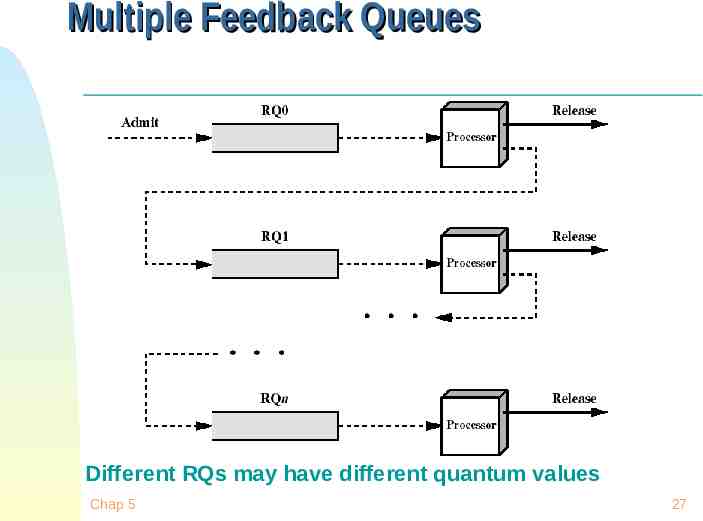
Multiple Feedback Queues Different RQs may have different quantum values Chap 5 27
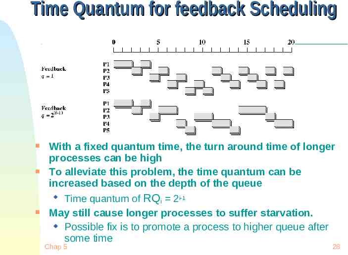
Time Quantum for feedback Scheduling With a fixed quantum time, the turn around time of longer processes can be high To alleviate this problem, the time quantum can be increased based on the depth of the queue Time quantum of RQ 2i-1 i May still cause longer processes to suffer starvation. Possible fix is to promote a process to higher queue after some time Chap 5 28
Algorithm Comparison Which one is the best? The answer depends on many factors: Chap 5 the system workload (extremely variable) hardware support for the dispatcher relative importance of performance criteria (response time, CPU utilization, throughput.) The evaluation method used (each has its limitations.) 29
Back to SJF: CPU Burst Estimation Let T[i] be the execution time for the ith instance of this process: the actual duration of the ith CPU burst of this process Let S[i] be the predicted value for the ith CPU burst of this process. The simplest choice is: S[n 1] (1/n)(T[1] T[n]) (1/n) {i 1 to n} T[i] This can be more efficiently calculated as: S[n 1] (1/n) T[n] ((n-1)/n) S[n] This estimate, however, results in equal weight for each instance Chap 5 30
Estimating the required CPU burst Recent instances are more likely to better reflect future behavior A common technique to factor the above observation into the estimate is to use exponential averaging : S[n 1] T[n] (1- ) S[n] ; Chap 5 0 1 31
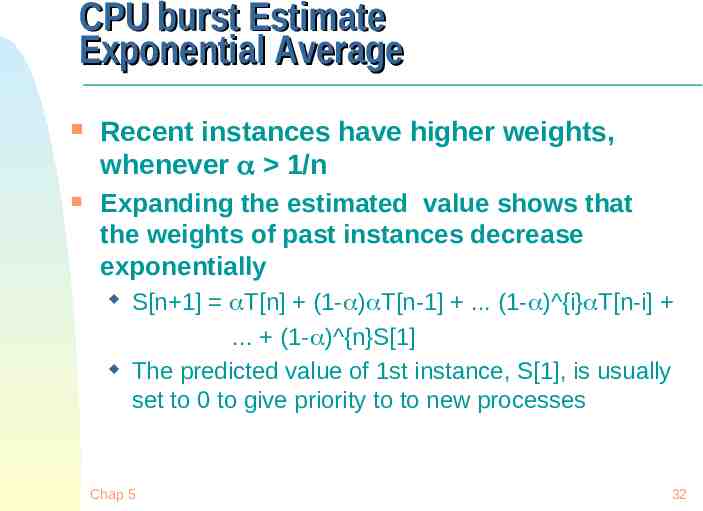
CPU burst Estimate Exponential Average Recent instances have higher weights, whenever 1/n Expanding the estimated value shows that the weights of past instances decrease exponentially S[n 1] T[n] (1- ) T[n-1] . (1- ) {i} T[n-i] . (1- ) {n}S[1] The predicted value of 1st instance, S[1], is usually set to 0 to give priority to to new processes Chap 5 32
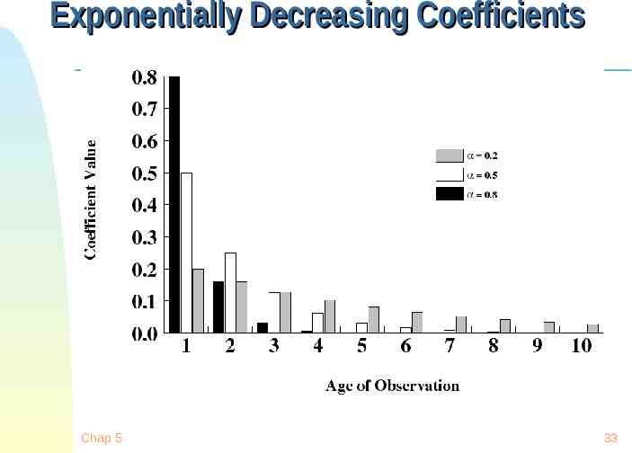
Exponentially Decreasing Coefficients Chap 5 33
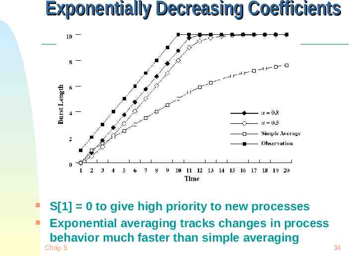
Exponentially Decreasing Coefficients S[1] 0 to give high priority to new processes Exponential averaging tracks changes in process behavior much faster than simple averaging Chap 5 34