Chapter 9: Trace Elements Note magnitud e of major element changes


95 Slides4.71 MB
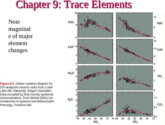
Chapter 9: Trace Elements Note magnitud e of major element changes Figure 8.2. Harker variation diagram for 310 analyzed volcanic rocks from Crater Lake (Mt. Mazama), Oregon Cascades. Data compiled by Rick Conrey (personal communication). From Winter (2001) An Introduction to Igneous and Metamorphic Petrology. Prentice Hall.
Chapter 9: Trace Elements Now note magnitud e of trace element changes Figure 9.1. Harker Diagram for Crater Lake. From data compiled by Rick Conrey. From Winter (2001) An Introduction to Igneous and Metamorphic Petrology. Prentice Hall.
Element Distribution Goldschmidt’s rules (simplistic, but useful) 1. 2 ions with the same valence and radius should exchange easily and enter a solid solution in amounts equal to their overall proportions How does Rb behave? Ni?
Goldschmidt’s rules 2. If 2 ions have a similar radius and the same valence: the smaller ion is preferentially incorporated into the solid over the liquid Fig. 6.10. Isobaric T-X phase diagram at atmospheric pressure After Bowen and Shairer (1932), Amer. J. Sci. 5th Ser., 24, 177-213. From Winter (2001) An Introduction to Igneous and Metamorphic Petrology. Prentice Hall.
3. If 2 ions have a similar radius, but different valence: the ion with the higher charge is preferentially incorporated into the solid over the liquid
Chemical Fractionation The uneven distribution of an ion between two competing (equilibrium) phases
Exchange equilibrium of a component i between two phases (solid and liquid) i (liquid) i (solid) ai ai liquid solid eq. 9.2 K K equilibrium constant i Xi solid X liquid i i
Trace element concentrations are in the Henry’s Law region of concentration, so their activity varies in direct relation to their concentration in the system Thus if XNi in the system doubles the XNi in all phases will double This does not mean that X in all phases Ni is the same, since trace elements do fractionate. Rather the XNi within each phase will vary in proportion to the system concentration
incompatible elements are concentrated in the melt (KD or D) « 1 compatible elements are concentrated in the solid KD or D » 1
For dilute solutions can substitute D for K D: CS D CL Where CS the concentration of some element in the solid phase
Incompatible elements commonly two subgroups Smaller, highly charged high field strength (HFS) elements (REE, Th, U, Ce, Pb4 , Zr, Hf, Ti, Nb, Ta) Low field strength large ion lithophile (LIL) elements (K, Rb, Cs, Ba, Pb2 , Sr, Eu2 ) are more mobile, particularly if a fluid phase is involved
Compatibility depends on minerals and melts involved. Which are incompatible? Why? Rb Sr Ba Ni Cr La Ce Nd Sm Eu Dy Er Yb Lu Rare Earth Elements Table 9-1. Partition Coefficients (CS/CL) for Some Commonly Used Trace Elements in Basaltic and Andesitic Rocks Olivine 0.01 0.014 0.01 14.0 0.7 0.007 0.006 0.006 0.007 0.007 0.013 0.026 0.049 0.045 Opx 0.022 0.04 0.013 5.0 10.0 0.03 0.02 0.03 0.05 0.05 0.15 0.23 0.34 0.42 Data from Rollinson (1993). Cpx Garnet 0.031 0.042 0.06 0.012 0.026 0.023 7.0 0.955 34.0 1.345 0.056 0.001 0.092 0.007 0.23 0.026 0.445 0.102 0.474 0.243 0.582 3.17 0.583 6.56 0.542 11.5 0.506 11.9 Plag Amph Magnetite 0.071 0.29 1.83 0.46 0.23 0.42 0.01 6.8 29. 0.01 2.0 7.4 0.148 0.544 2. 0.082 0.843 2. 0.055 1.34 2. 0.039 1.804 1. 0.1/1.5* 1.557 1. 0.023 2.024 1. 0.02 1.74 1.5 0.023 1.642 1.4 0.019 1.563 * Eu3 /Eu2 Italics are estimated
For a rock, determine the bulk distribution coefficient D for an element by calculating the contribution for each mineral eq. 9.4: Di WA Di A WA weight % of mineral A in the rock DiA partition coefficient of element i in mineral A
Rb Sr Ba Ni Cr La Ce Nd Sm Eu Dy Er Yb Lu Rare Earth Elements Table 9-1. Partition Coefficients (CS/CL) for Some Commonly Used Trace Elements in Basaltic and Andesitic Rocks Olivine 0.010 0.014 0.010 14 0.70 0.007 0.006 0.006 0.007 0.007 0.013 0.026 0.049 0.045 Opx 0.022 0.040 0.013 5 10 0.03 0.02 0.03 0.05 0.05 0.15 0.23 0.34 0.42 Data from Rollinson (1993). Cpx Garnet 0.031 0.042 0.060 0.012 0.026 0.023 7 0.955 34 1.345 0.056 0.001 0.092 0.007 0.230 0.026 0.445 0.102 0.474 0.243 0.582 1.940 0.583 4.700 0.542 6.167 0.506 6.950 Plag Amph Magnetite 0.071 0.29 1.830 0.46 0.23 0.42 0.01 6.8 29 0.01 2.00 7.4 0.148 0.544 2 0.082 0.843 2 0.055 1.340 2 0.039 1.804 1 0.1/1.5* 1.557 1 0.023 2.024 1 0.020 1.740 1.5 0.023 1.642 1.4 0.019 1.563 * Eu3 /Eu2 Italics are estimated Example: hypothetical garnet lherzolite 60% olivine, 25% orthopyroxene, 10% clinopyroxene, and 5% garnet (all by weight), using the data in Table 9.1, is: DEr (0.6 · 0.026) (0.25 · 0.23) (0.10 · 0.583) (0.05 · 4.7) 0.366
Trace elements strongly partitioned into a single mineral Ni - olivine in Table 9.1 14 Figure 9.1a. Ni Harker Diagram for Crater Lake. From data compiled by Rick Conrey. From Winter (2001) An Introduction to Igneous and Metamorphic Petrology. Prentice Hall.
Incompatible trace elements concentrate liquid Reflect the proportion of liquid at a given state of crystallization or melting Figure 9.1b. Zr Harker Diagram for Crater Lake. From data compiled by Rick Conrey. From Winter (2001) An Introduction to Igneous and Metamorphic Petrology. Prentice Hall.
Trace Element Behavior The concentration of a major element in a phase is usually buffered by the system, so that it varies little in a phase as the system composition changes At a given T we could vary Xbulk from 35 70 % Mg/Fe without changing the composition of the melt or the olivine
Trace element concentrations are in the Henry’s Law region of concentration, so their activity varies in direct relation to their concentration in the system
Trace element concentrations are in the Henry’s Law region of concentration, so their activity varies in direct relation to their concentration in the system Thus if XNi in the system doubles the XNi in all phases will double
Trace element concentrations are in the Henry’s Law region of concentration, so their activity varies in direct relation to their concentration in the system Thus if XNi in the system doubles the XNi in all phases will double Because of this, the ratios of trace elements are often superior to the concentration of a single element in identifying the role of a specific mineral
K/Rb often used the importance of amphibole in a source rock K & Rb behave very similarly, so K/Rb should be constant If amphibole, almost all K and Rb reside in it Amphibole has a D of about 1.0 for K and 0.3 for Rb Table 9-1. Partition Coefficients (CS/CL) for Some Commonly Used Trace Elements in Basaltic and Andesitic Rocks Rb Sr Ba Ni Cr La Ce Nd Sm Eu Dy Er Yb Lu Rare Earth Elements Olivine 0.010 0.014 0.010 14 0.70 0.007 0.006 0.006 0.007 0.007 0.013 0.026 0.049 0.045 Opx 0.022 0.040 0.013 5 10 0.03 0.02 0.03 0.05 0.05 0.15 0.23 0.34 0.42 Data from Rollinson (1993). Cpx Garnet 0.031 0.042 0.060 0.012 0.026 0.023 7 0.955 34 1.345 0.056 0.001 0.092 0.007 0.230 0.026 0.445 0.102 0.474 0.243 0.582 1.940 0.583 4.700 0.542 6.167 0.506 6.950 Plag Amph Magnetite 0.071 0.29 1.830 0.46 0.23 0.42 0.01 6.8 29 0.01 2.00 7.4 0.148 0.544 2 0.082 0.843 2 0.055 1.340 2 0.039 1.804 1 0.1/1.5* 1.557 1 0.023 2.024 1 0.020 1.740 1.5 0.023 1.642 1.4 0.019 1.563 * Eu3 /Eu2 Italics are estimated
Sr and Ba (also incompatible elements) Sr is excluded from most common minerals except plagioclase Ba similarly excluded except in alkali feldspar Table 9-1. Partition Coefficients (CS/CL) for Some Commonly Used Trace Elements in Basaltic and Andesitic Rocks Rb Sr Ba Ni Cr La Ce Nd Sm Eu Dy Er Yb Lu Rare Earth Elements Olivine 0.010 0.014 0.010 14 0.70 0.007 0.006 0.006 0.007 0.007 0.013 0.026 0.049 0.045 Opx 0.022 0.040 0.013 5 10 0.03 0.02 0.03 0.05 0.05 0.15 0.23 0.34 0.42 Data from Rollinson (1993). Cpx Garnet 0.031 0.042 0.060 0.012 0.026 0.023 7 0.955 34 1.345 0.056 0.001 0.092 0.007 0.230 0.026 0.445 0.102 0.474 0.243 0.582 1.940 0.583 4.700 0.542 6.167 0.506 6.950 Plag Amph Magnetite 0.071 0.29 1.830 0.46 0.23 0.42 0.01 6.8 29 0.01 2.00 7.4 0.148 0.544 2 0.082 0.843 2 0.055 1.340 2 0.039 1.804 1 0.1/1.5* 1.557 1 0.023 2.024 1 0.020 1.740 1.5 0.023 1.642 1.4 0.019 1.563 * Eu3 /Eu2 Italics are estimated
Compatible example: Ni strongly fractionated olivine pyroxene Cr and Sc pyroxenes » olivine Ni/Cr or Ni/Sc can distinguish the effects of olivine and augite in a partial melt or a suite of rocks produced by fractional crystallization
Models of Magma Evolution Batch Melting The melt remains resident until at some point it is released and moves upward Equilibrium melting process with variable % melting
Models of Magma Evolution Batch Melting 1 eq. 9.5 CL CO Di(1 F) F CL trace element concentration in the liquid CO trace element concentration in the original rock before melting began F wt fraction of melt produced melt/(melt rock)
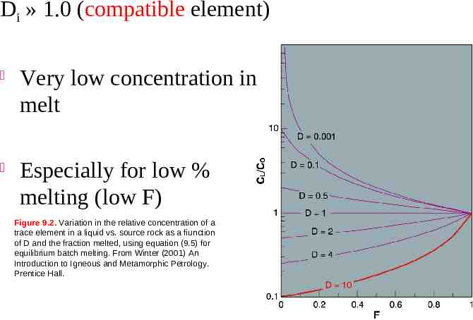
Batch Melting A plot of CL/CO vs. F for various values of Di using eq. 9.5 Di 1.0 Figure 9.2. Variation in the relative concentration of a trace element in a liquid vs. source rock as a fiunction of D and the fraction melted, using equation (9.5) for equilibrium batch melting. From Winter (2001) An Introduction to Igneous and Metamorphic Petrology. Prentice Hall.
Di » 1.0 (compatible element) Very low concentration in melt Especially for low % melting (low F) Figure 9.2. Variation in the relative concentration of a trace element in a liquid vs. source rock as a fiunction of D and the fraction melted, using equation (9.5) for equilibrium batch melting. From Winter (2001) An Introduction to Igneous and Metamorphic Petrology. Prentice Hall.
Highly incompatible elements Greatly concentrated in the initial small fraction of melt produced by partial melting Subsequently diluted as F increases Figure 9.2. Variation in the relative concentration of a trace element in a liquid vs. source rock as a fiunction of D and the fraction melted, using equation (9.5) for equilibrium batch melting. From Winter (2001) An Introduction to Igneous and Metamorphic Petrology. Prentice Hall.
As F 1 the concentration of every trace element in the liquid the source rock (CL/CO 1) 1 CL C O Di (1 1F) F As F CL/CO 1 Figure 9.2. Variation in the relative concentration of a trace element in a liquid vs. source rock as a fiunction of D and the fraction melted, using equation (9.5) for equilibrium batch melting. From Winter (2001) An Introduction to Igneous and Metamorphic Petrology. Prentice Hall.
As F 0 CL/CO 1/Di 1 CL C O Di (1 F) F If we know CL of a magma derived by a small degree of batch melting, and we know Di we can estimate the concentration of that element in the source region (CO) Figure 9.2. Variation in the relative concentration of a trace element in a liquid vs. source rock as a fiunction of D and the fraction melted, using equation (9.5) for equilibrium batch melting. From Winter (2001) An Introduction to Igneous and Metamorphic Petrology. Prentice Hall.
For very incompatible elements as Di 0 equation 9.5 to: eq. 9.7 1 CL C O Di (1 F) F reduces CL 1 CO F If we know the concentration of a very incompatible element in both a magma and the source rock, we can determine the fraction of partial melt produced
Worked Example of Batch Melting: Rb and Sr with the mode: Basalt Table 9.2. Conversion from mode to weight percent Mineral Mode Density Wt prop Wt% ol 15 3.6 54 0.18 cpx 33 3.4 112.2 0.37 plag 51 2.7 137.7 0.45 Sum 303.9 1.00 1. Convert to weight % minerals (Wol Wcpx etc.)
Worked Example of Batch Melting: Rb and Sr with the mode: Basalt Table 9.2. Conversion from mode to weight percent Mineral Mode Density Wt prop Wt% ol 15 3.6 54 0.18 cpx 33 3.4 112.2 0.37 plag 51 2.7 137.7 0.45 Sum 303.9 1.00 1. Convert to weight % minerals (Wol Wcpx etc.) 2. Use equation eq. 9.4: Di WA Di and the table of D values for Rb and Sr in each mineral to calculate the bulk distribution coefficients: DRb 0.045 and D 0.848
3. Use the batch melting equation (9.5) 1 CL C O Di (1 F) F to calculate CL/CO for various values of F Table 9.3 . Batch Fractionation Model for Rb and Sr F 0.05 0.1 0.15 0.2 0.3 0.4 0.5 0.6 0.7 0.8 0.9 C L/C O 1/(D(1-F) F) D Rb D Sr 0.045 0.848 9.35 1.14 6.49 1.13 4.98 1.12 4.03 1.12 2.92 1.10 2.29 1.08 1.89 1.07 1.60 1.05 1.39 1.04 1.23 1.03 1.10 1.01 Rb/Sr 8.19 5.73 4.43 3.61 2.66 2.11 1.76 1.52 1.34 1.20 1.09 From Winter (2010) An Introduction to Igneous and Metamorphic Petrology. Prentice Hall.
4. Plot CL/CO vs. F for each element Figure 9.3. Change in the concentration of Rb and Sr in the melt derived by progressive batch melting of a basaltic rock consisting of plagioclase, augite, and olivine. From Winter (2001) An Introduction to Igneous and Metamorphic Petrology. Prentice Hall.
Incremental Batch Melting Calculate batch melting for successive batches (same equation) Must recalculate Di as solids change as minerals are selectively melted (computer)
Fractional Crystallization 1. Crystals remain in equilibrium with each melt increment
Rayleigh fractionation The other extreme: separation of each crystal as it formed perfectly continuous fractional crystallization in a magma chamber
Rayleigh fractionation The other extreme: separation of each crystal as it formed perfectly continuous fractional crystallization in a magma chamber Concentration of some element in the residual liquid, CL is modeled by the Rayleigh equation: eq. 9.8 CL/CO F (D -1) Rayleigh Fractionation
Other models are used to analyze Mixing of magmas Wall-rock assimilation Zone refining Combinations of processes
The Rare Earth Elements (REE)
Contrasts and similarities in the D values: All are incompatible HREE are less incompatible Especially in garnet Eu can 2 which conc. in plagioclase Rb Sr Ba Ni Cr La Ce Nd Sm Eu Dy Er Yb Lu Rare Earth Elements Also Note: Table 9-1. Partition Coefficients (CS/CL) for Some Commonly Used Trace Elements in Basaltic and Andesitic Rocks Olivine 0.01 0.014 0.01 14.0 0.7 0.007 0.006 0.006 0.007 0.007 0.013 0.026 0.049 0.045 Opx 0.022 0.04 0.013 5.0 10.0 0.03 0.02 0.03 0.05 0.05 0.15 0.23 0.34 0.42 Data from Rollinson (1993). Cpx Garnet 0.031 0.042 0.06 0.012 0.026 0.023 7.0 0.955 34.0 1.345 0.056 0.001 0.092 0.007 0.23 0.026 0.445 0.102 0.474 0.243 0.582 3.17 0.583 6.56 0.542 11.5 0.506 11.9 Plag Amph Magnetite 0.071 0.29 1.83 0.46 0.23 0.42 0.01 6.8 29. 0.01 2.0 7.4 0.148 0.544 2. 0.082 0.843 2. 0.055 1.34 2. 0.039 1.804 1. 0.1/1.5* 1.557 1. 0.023 2.024 1. 0.02 1.74 1.5 0.023 1.642 1.4 0.019 1.563 * Eu3 /Eu2 Italics are estimated
REE Diagrams Plots of concentration as the ordinate (y-axis) against increasing atomic number Degree of compatibility increases from left to right across the diagram (“lanthanide contraction”) Concentration La Ce Nd Sm Eu Tb Er Dy Yb Lu
Log (Abundance in CI Chondritic Meteorite) 11 H He 10 9 8 C 7 6 5 4 3 2 1 Li O Ne MgSi Fe N S Ar Ca Ni Na Ti AlP K F Cl V B Sc Sn Ba Pt Pb 0 Be -1 Th -2 U -3 0 10 20 30 40 50 60 70 80 90 Atomic Number (Z) Eliminate Oddo-Harkins effect and make y-scale more functional by normalizing to a standard estimates of primordial mantle REE chondrite meteorite concentrations 100
What would an REE diagram look like for an analysis of a chondrite meteorite? sample/chondrite 10.00 8.00 6.00 ? 4.00 2.00 0.00 56 La58 Ce L 60Nd 62Sm 64 Eu 66 Tb 68Er 70 Yb 72 Lu
Divide each element in analysis by the concentration in a chondrite standard sample/chondrite 10.00 8.00 6.00 4.00 2.00 0.00 56 La58 Ce L 60Nd 62Sm 64 Eu 66 Tb 68Er 70 Yb 72 Lu
REE diagrams using batch melting model of a garnet lherzolite for various values of F: Figure 9.4. Rare Earth concentrations (normalized to chondrite) for melts produced at various values of F via melting of a hypothetical garnet lherzolite using the batch melting model (equation 9.5). From Winter (2001) An Introduction to Igneous and Metamorphic Petrology. Prentice Hall.
Europium anomaly when plagioclase is a fractionating phenocryst or a residual solid in source Figure 9.5. REE diagram for 10% batch melting of a hypothetical lherzolite with 20% plagioclase, resulting in a pronounced negative Europium anomaly. From Winter (2001) An Introduction to Igneous and Metamorphic Petrology. Prentice Hall.
Normalized Multielement (Spider) Diagrams An extension of the normalized REE technique to a broader spectrum of elements Chondrite-normalized spider diagrams are commonly organized by (the author’s estimate) of increasing incompatibility L R Different estimates different ordering (poor standardization) Fig. 9.6. Spider diagram for an alkaline basalt from Gough Island, southern Atlantic. After Sun and MacDonough (1989). In A. D. Saunders and M. J. Norry (eds.), Magmatism in the Ocean Basins. Geol. Soc. London Spec. Publ., 42. pp. 313-345.
MORB-normalized Spider Separates LIL and HFS Figure 9.7. Ocean island basalt plotted on a mid-ocean ridge basalt (MORB) normalized spider diagram of the type used by Pearce (1983). Data from Sun and McDonough (1989). From Winter (2001) An Introduction to Igneous and Metamorphic Petrology. Prentice Hall.
Application of Trace Elements to Igneous Systems 1. Use like major elements on variation diagrams to document FX, assimilation, etc. in a suite of rocks More sensitive larger variations as process continues Figure 9.1a. Ni Harker Diagram for Crater Lake. From data compiled by Rick Conrey. From Winter (2001) An Introduction to Igneous and Metamorphic Petrology. Prentice Hall.
2. Identification of the source rock or a particular mineral involved in either partial melting or fractional crystallization processes
Garnet concentrates the HREE and fractionates among them Thus if garnet is in equilibrium with the partial melt (a residual phase in the source left behind) expect a steep (-) slope in REE and HREE Shallow ( 40 km) partial melting of the mantle will have plagioclase in the resuduum and a Eu anomaly will result Rb Sr Ba Ni Cr La Ce Nd Sm Eu Dy Er Yb Lu Rare Earth Elements Table 9-1. Partition Coefficients (CS/CL) for Some Commonly Used Trace Elements in Basaltic and Andesitic Rocks Olivine 0.01 0.014 0.01 14.0 0.7 0.007 0.006 0.006 0.007 0.007 0.013 0.026 0.049 0.045 Opx 0.022 0.04 0.013 5.0 10.0 0.03 0.02 0.03 0.05 0.05 0.15 0.23 0.34 0.42 Data from Rollinson (1993). Cpx Garnet 0.031 0.042 0.06 0.012 0.026 0.023 7.0 0.955 34.0 1.345 0.056 0.001 0.092 0.007 0.23 0.026 0.445 0.102 0.474 0.243 0.582 3.17 0.583 6.56 0.542 11.5 0.506 11.9 Plag Amph Magnetite 0.071 0.29 1.83 0.46 0.23 0.42 0.01 6.8 29. 0.01 2.0 7.4 0.148 0.544 2. 0.082 0.843 2. 0.055 1.34 2. 0.039 1.804 1. 0.1/1.5* 1.557 1. 0.023 2.024 1. 0.02 1.74 1.5 0.023 1.642 1.4 0.019 1.563 * Eu3 /Eu2 Italics are estimated
10.00 67% Ol sample/chondrite 8.00 17% Opx 17% Cpx Garnet and Plagioclase effect on HREE 6.00 4.00 2.00 0.00 56 58 Ce 60 Nd 62Sm Eu 64 La Tb66 68 Er 70 Lu 72 Yb 10.00 10.00 60% Ol 15% Opx 15% Cpx 10%Plag sample/chondrite sample/chondrite 8.00 6.00 4.00 57% Ol 8.00 14% Opx 14% Cpx 14% Grt 6.00 4.00 2.00 2.00 0.00 0.00 La Ce Nd Sm Eu Tb Er Yb Lu 56 58 La 64 Ce60 Nd 62Sm Eu Tb66 68 Er 70 Lu Yb 72
Figure 9.3. Change in the concentration of Rb and Sr in the melt derived by progressive batch melting of a basaltic rock consisting of plagioclase, augite, and olivine. From Winter (2001) An Introduction to Igneous and Metamorphic Petrology. Prentice Hall.
Table 9.6 A Brief Summary of Some Particularly Useful Trace Elements in Igneous Petrology Element Ni, Co, Cr Use as a Petrogenetic Indicator Highly compatible elements. Ni and Co are concentrated in olivine, and Cr in spinel and clinopyroxene. High concentrations indicate a mantle source, limited fractionation, or crystal accumulation. Zr, Hf Very incompatible elements that do not substitute into major silicate phases (although they may replace Ti in titanite or rutile). High concentrations imply an enriched source or extensive liquid evolution. Nb, Ta High field-strength elements that partition into Ti-rich phases (titanite, Ti-amphibole, Fe-Ti oxides. Typically low concentrations in subduction-related melts. Ru, Rh, Pd, Platinum group elements (PGEs) are siderophile and used mostly to study melting and crystallization in mafic-ultramafic Re, Os, Ir, systems in which PGEs are typically hosted by sulfides. The Re/Os isotopic system is controlled by initial PGE Pd differentiation and is applied to mantle evolution and mafic melt processes. Sc Concentrates in pyroxenes and may be used as an indicator of pyroxene fractionation. Sr Substitutes for Ca in plagioclase (but not in pyroxene), and, to a lesser extent, for K in K-feldspar. Behaves as a compatible element at low pressure where plagioclase forms early, but as an incompatible element at higher pressure where plagioclase is no longer stable. REE Myriad uses in modeling source characteristics and liquid evolution. Garnet accommodates the HREE more than the LREE, and orthopyroxene and hornblende do so to a lesser degree. Titanite and plagioclase accommodates more LREE. Eu2 is strongly partitioned into plagioclase. Y Commonly incompatible. Strongly partitioned into garnet and amphibole. Titanite and apatite also concentrate Y, so the presence of these as accessories could have a significant effect.
Trace elements as a tool to determine paleotectonic environment Useful for rocks in mobile belts that are no longer recognizably in their original setting Can trace elements be discriminators of igneous environment? Approach is empirical on modern occurrences Concentrate on elements that are immobile during low/medium grade metamorphism
Figure 9.8 Examples of discrimination diagrams used to infer tectonic setting of ancient (meta)volcanics. (a) after Pearce and Cann (1973), (b) after Pearce (1982), Coish et al. (1986). Reprinted by permission of the American Journal of Science, (c) after Mullen (1983) Copyright with permission from Elsevier Science, (d) and (e) after Vermeesch (2005) AGU with permission.
Isotopes Same Z, different A (variable # of neutrons) 14 General notation for a nuclide: 6C
Isotopes Same Z, different A (variable # of neutrons) 14 General notation for a nuclide: 6 C As n varies different isotopes of an element 12 C 13 C 14 C
Stable Isotopes Stable: last forever Chemical fractionation is impossible Mass fractionation is the only type possible
Example: Oxygen Isotopes O oxygen 17 O 18 O 16 99.756% of natural 0.039% 0.205% “ “ Concentrations expressed by reference to a standard International standard for O isotopes standard mean ocean water (SMOW)
18 O and 16O are the commonly used isotopes and their ratio is expressed as : 18O/16O) eq 18 16 18 16 ( O/ O) sample ( O/ O) SMOW 18 16 ( O/ O) SMOW result expressed in per mille (‰) What is of SMOW? What is for meteoric water? x1000
What is for meteoric water? Evaporation seawater water vapor (clouds) Light isotope enriched in vapor liquid Pretty efficient, since mass 1/8 total mass
What is for meteoric water? Evaporation seawater water vapor (clouds) Light isotope enriched in vapor liquid Pretty efficient, since mass 1/8 total mass ( 18 O/ 16 O) vapor ( 18 O/ 16 O) SMOW 18 16 ( O/ O) SMOW 18 16 ( O/ therefore O) Vapor thus clouds is (-) x 1000 16 ( 18 O/ O) SMOW
Figure 9.9. Relationship between d(18O/16O) and mean annual temperature for meteoric precipitation, after Dansgaard (1964). Tellus, 16, 436-468.
Stable isotopes useful in assessing relative contribution of various reservoirs, each with a distinctive isotopic signature O and H isotopes - juvenile vs. meteoric vs. brine water 18O for mantle rocks surface-reworked sediments: evaluate contamination of mantlederived magmas by crustal sediments
Radioactive Isotopes Unstable isotopes decay to other nuclides The rate of decay is constant, and not affected by P, T, X Parent nuclide radioactive nuclide that decays Daughter nuclide(s) are the radiogenic atomic products
Isotopic variations between rocks, etc. due to: 1. Mass fractionation (as for stable isotopes) Only effective for light isotopes: H He C O S
Isotopic variations between rocks, etc. due to: 1. Mass fractionation (as for stable isotopes) 2. Daughters produced in varying proportions resulting from previous event of chemical fractionation K 40Ar by radioactive decay 40 Basalt rhyolite by FX (a chemical fractionation process) Rhyolite has more K than basalt K more 40Ar over time in rhyolite than in basalt 40 Ar/39Ar ratio will be different in each 40
Isotopic variations between rocks, etc. due to: 1. Mass fractionation (as for stable isotopes) 2. Daughters produced in varying proportions resulting from previous event of chemical fractionation 3. Time The longer 40K 40Ar decay takes place, the greater the difference between the basalt and rhyolite will be
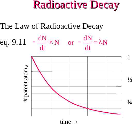
Radioactive Decay The Law of Radioactive Decay eq. 9.11 dN N dt or dN N dt # parent atoms 1 ½ ¼ time
D Ne t - N N(e t -1) eq 9.14 age of a sample (t) if we know: D the amount of the daughter nuclide produced N the amount of the original parent nuclide remaining the decay constant for the system in question
The K-Ar System 40 K either 40Ca or 40Ar Ca is common. Cannot distinguish radiogenic 40 Ca from non-radiogenic 40Ca 40 Ar is an inert gas which can be trapped in many solid phases as it forms in them 40
The appropriate decay equation is: eq 9.16 e 40 Ar 40Aro 40 K(e- t -1) Where e 0.581 x 10⁻¹⁰ a-1 (proton capture) and 5.543 x 10⁻¹⁰ a-1 (whole process)
Blocking temperatures for various minerals differ 40 Ar-39Ar technique grew from this discovery
Sr-Rb System 87 Rb 87Sr a beta particle ( 1.42 x 10⁻¹¹ a-1) Rb behaves like K micas and alkali feldspar Sr behaves like Ca plagioclase and apatite (but not clinopyroxene) 88 Sr : 87Sr : 86Sr : 84Sr ave. sample 10 : 0.7 : 1 : 0.07 86 Sr is a stable isotope, and not created by breakdown of any other parent
Isochron Technique Requires 3 or more cogenetic samples with a range of Rb/Sr Could be: 3 cogenetic rocks derived from a single source by partial melting, FX, etc. Figure 9.3. Change in the concentration of Rb and Sr in the melt derived by progressive batch melting of a basaltic rock consisting of plagioclase, augite, and olivine. From Winter (2001) An Introduction to Igneous and Metamorphic Petrology. Prentice Hall.
Isochron Technique Requires 3 or more cogenetic samples with a range of Rb/Sr Could be: 3 cogenetic rocks derived from a single source by partial melting, FX, etc. 3 coexisting minerals with different K/Ca ratios in a single rock
Recast age equation by dividing through by stable 86Sr 87 Sr/86Sr (87Sr/86Sr)o (87Rb/86Sr)(e t -1) eq 9.17 1.4 x 10⁻¹¹ a-1 For values of t less than 0.1: e t-1 t Thus eq. 9.15 for t 70 Ga (!!) reduces to: eq 9.18 87 Sr/86Sr (87Sr/86Sr)o (87Rb/86Sr) t y b m equation for a line in 87Sr/86Sr vs. 87Rb/86Sr plot x
Begin with 3 rocks plotting at a b c at time to Sr 86 Sr 87 ( ) Sr Sr 87 86 o a b Rb 86 Sr 87 c to
After some time increment (t0 t1) each sample loses some 87Rb and gains an equivalent amount of 87Sr Sr 86 Sr 87 () Sr Sr c1 b1 a1 t1 87 86 o a b Rb 86 Sr 87 c to
At time t2 each rock system has evolved new line Again still linear and steeper line t2 Sr 86 Sr 87 c2 b2 a2 () Sr Sr c1 b1 a1 t1 87 86 o a b c to Rb 86 Sr 87
Isochron technique produces 2 valuable things: 1. The age of the rocks (from the slope t) 2. (87Sr/86Sr)o the initial value of 87Sr/86Sr Figure 9.12. Rb-Sr isochron for the Eagle Peak Pluton, central Sierra Nevada Batholith, California, USA. Filled circles are whole-rock analyses, open circles are hornblende separates. The regression equation for the data is also given. After Hill et al. (1988). Amer. J. Sci., 288-A, 213-241.
Figure 9.13. Estimated Rb and Sr isotopic evolution of the Earth’s upper mantle, assuming a large-scale melting event producing granitic-type continental rocks at 3.0 Ga b.p After Wilson (1989). Igneous Petrogenesis. Unwin Hyman/Kluwer.
The Sm-Nd System Both Sm and Nd are LREE Incompatible elements fractionate melts Nd has lower Z larger liquids does Sm
147 Sm 143Nd by alpha decay 6.54 x 10⁻¹³ a-1 (half life 106 Ga) Decay equation derived by reference to the non-radiogenic 144Nd 143Nd/144Nd (143Nd/144Nd) o (147Sm/144Nd) t
Evolution curve is opposite to Rb - Sr Figure 9.15. Estimated Nd isotopic evolution of the Earth’s upper mantle, assuming a large-scale melting or enrichment event at 3.0 Ga b.p. After Wilson (1989). Igneous Petrogenesis. Unwin Hyman/Kluwer.
The U-Pb-Th System Very complex system. 3 radioactive isotopes of U: 234U, 235U, 238U 3 radiogenic isotopes of Pb: 206Pb, 207Pb, and 208Pb Only 204Pb is strictly non-radiogenic U, Th, and Pb are incompatible elements, & concentrate in early melts Isotopic composition of Pb in rocks function of U 234U 206Pb 235 U 207Pb 232 Th 208Pb 238 ( 1.5512 x 10⁻¹⁰ a-1) ( 9.8485 x 10⁻¹⁰ a-1) ( 4.9475 x 10⁻¹¹ a-1)
The U-Pb-Th System Concordia Simultaneous coevolution of 206Pb and 207Pb via: U 234U 206Pb 235 U 207Pb 238 Figure 9.16a. Concordia diagram illustrating the Pb isotopic development of a 3.5 Ga old rock with a single episode of Pb loss. After Faure (1986). Principles of Isotope Geology. 2nd, ed. John Wiley & Sons. New York.
The U-Pb-Th System Discordia loss of both 206 Pb and 207Pb Figure 9.16a. Concordia diagram illustrating the Pb isotopic development of a 3.5 Ga old rock with a single episode of Pb loss. After Faure (1986). Principles of Isotope Geology. 2nd, ed. John Wiley & Sons. New York.
The U-Pb-Th System Concordia diagram after 3.5 Ga total evolution Figure 9.16b. Concordia diagram illustrating the Pb isotopic development of a 3.5 Ga old rock with a single episode of Pb loss. After Faure (1986). Principles of Isotope Geology. 2nd, ed. John Wiley & Sons. New York.
The U-Pb-Th System Figure 9.17. Concordia diagram for three discordant zircons separated from an Archean gneiss at Morton and Granite Falls, Minnesota. The discordia intersects the concordia at 3.55 Ga, yielding the U-Pb age of the gneiss, and at 1.85 Ga, yielding the U-Pb age of the depletion event. From Faure (1986). Copyright reprinted by permission of John Wiley & Sons, Inc.