BIRCH: Balanced Iterative Reducing and Clustering Using Hierarchies


30 Slides1,005.50 KB
BIRCH: Balanced Iterative Reducing and Clustering Using Hierarchies A hierarchical clustering method. It introduces two concepts : Clustering feature Clustering feature tree (CF tree) These structures help the clustering method achieve good speed and scalability in large databases.
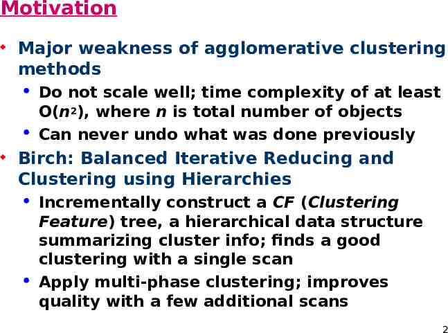
Motivation Major weakness of agglomerative clustering methods Do not scale well; time complexity of at least O(n2), where n is total number of objects Can never undo what was done previously Birch: Balanced Iterative Reducing and Clustering using Hierarchies Incrementally construct a CF (Clustering Feature) tree, a hierarchical data structure summarizing cluster info; finds a good clustering with a single scan Apply multi-phase clustering; improves quality with a few additional scans 2
Summarized Info for Single cluster Given a cluster with N objects N X Centroid i 1 i X0 N Radius R ( N ( X X ) i 0 i 1 N Diameter N N i 1 j 1 D ( 2 ) (Xi X j ) N ( N 1) 1/ 2 2 1/ 2 ) 3
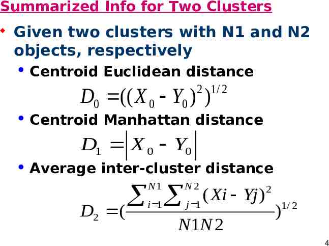
Summarized Info for Two Clusters Given two clusters with N1 and N2 objects, respectively Centroid Euclidean distance Centroid Manhattan distance Average inter-cluster distance 2 1/ 2 D0 (( X 0 Y0 ) ) D1 X 0 Y0 2 i 1 j 1 ( Xi Yj ) N1 D2 ( N2 N1N 2 )1/ 2 4
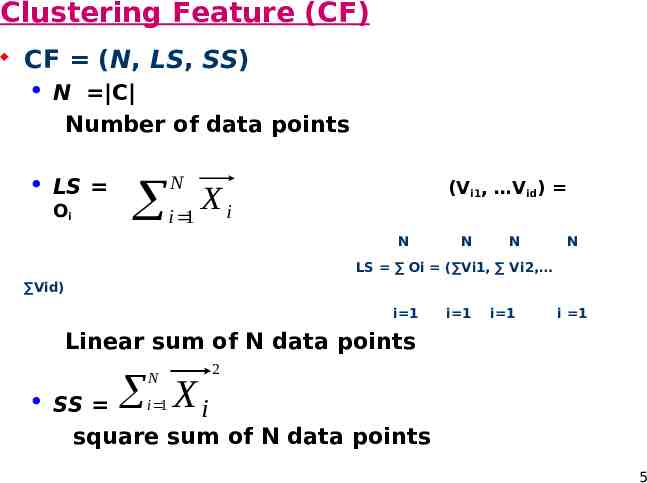
Clustering Feature (CF) CF (N, LS, SS) N C Number of data points LS Oi N i 1 (Vi1, Vid) Xi N N N N LS Oi ( Vi1, Vi2, Vid) i 1 i 1 i 1 i 1 Linear sum of N data points N X 2 i 1 SS i square sum of N data points 5
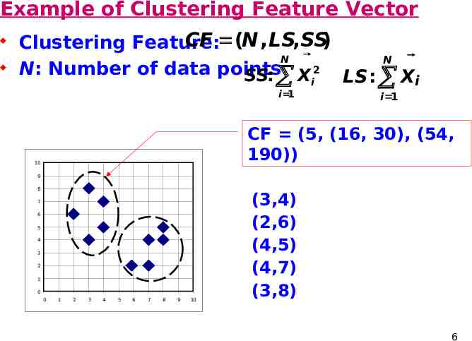
Example of Clustering Feature Vector Clustering Feature: CF (N , LS,SS) N 2 N: Number of data points SS: Xi i 1 N LS : Xi i 1 CF (5, (16, 30), (54, 190)) 10 9 8 7 6 5 4 3 2 1 0 0 1 2 3 4 5 6 7 8 9 10 (3,4) (2,6) (4,5) (4,7) (3,8) 6
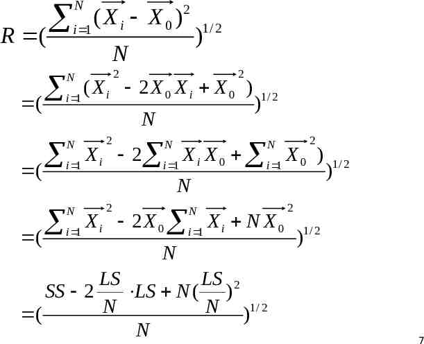
R ( ( ( ( N i 1 (Xi X0) 2 1/ 2 ) N 2 N 2 ( X 2 X X X ) i 0 i 0 i 1 N N i 1 2 )1/ 2 N 2 N X i 2 i 1 X i X 0 i 1 X 0 ) N N i 1 2 N X i 2 X 0 i 1 X i N X 0 N LS LS 2 SS 2 LS N ( ) N N )1/ 2 ( N )1/ 2 2 1/ 2 ) 7
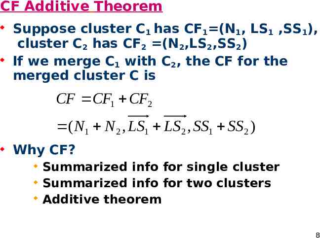
CF Additive Theorem Suppose cluster C1 has CF1 (N1, LS1 ,SS1), cluster C2 has CF2 (N2,LS2,SS2) If we merge C1 with C2, the CF for the merged cluster C is CF CF1 CF2 ( N1 N 2 , LS1 LS 2 , SS1 SS 2 ) Why CF? Summarized info for single cluster Summarized info for two clusters Additive theorem 8
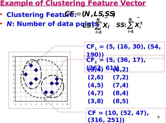
Example of Clustering Feature Vector Clustering Feature: CF (N , LS,SS) N N: Number of data points LS : Xi i 1 N 2 SS: Xi i 1 CF1 (5, (16, 30), (54, 190)) CF2 (5, (36, 17), (262, (3,4) 61)) (6,2) 10 9 8 7 6 5 4 3 2 1 0 0 1 2 3 4 5 6 7 8 9 10 (2,6) (4,5) (4,7) (3,8) (7,2) (7,4) (8,4) (8,5) CF (10, (52, 47), (316, 251)) 9
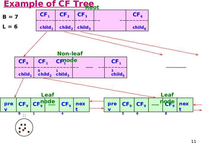
Clustering Feature Tree (CFT) Clustering feature tree (CFT) is an alternative representation of data set: Each non-leaf node is a cluster comprising sub-clusters corresponding to entries (at most B) in non-leaf node Each leaf node is a cluster comprising subclusters corresponding to entries (at most L) in leaf node and each sub-cluster’s diameter is at most T; when T is larger, CFT is smaller Each node must fit a memory page 10
Example of CF Tree Root B 7 CF1 CF2 CF3 CF6 L 6 child1 child2 child3 child6 CF9 child1 pre v CF1 Non-leaf CFnode 1 CF1 0 1 3 child2 child3 child5 CF9 Leaf node CF9 CF9 nex 0 1 4 t pre v CF9 CF9 5 6 Leaf node nex CF9 8 t 11
BIRCH Phase 1 Phase 1 scans data points and build inmemory CFT; Start from root, traverse down tree to choose closest leaf node for d Search for closest entry Li in leaf node If d can be inserted in Li, then update CF vector of Li Else if node has space to insert new entry, insert; else split node Once inserted, update nodes along path to the root; if there is splitting, need to insert new entry in parent node (which may result in further splitting) 12
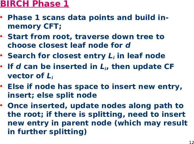
Example of the BIRCH Algorithm New subcluster sc8 sc3 sc1 sc4 sc2 sc5 sc7 sc6 LN3 LN2 Root LN1 LN1 sc8 LN2 LN3 sc5 sc6 sc1 sc2 sc3 sc4 sc7 13
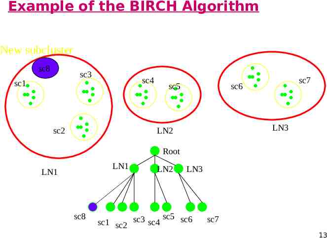
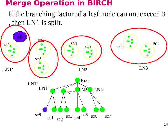
Merge Operation in BIRCH If the branching factor of a leaf node can not exceed 3 , then LN1 is split. sc8 sc1 sc3 sc4 sc5 sc7 sc6 sc2 LN1’ LN3 LN2 LN1” Root LN1’ sc8 LN1” LN2 LN3 sc5 sc6 sc1 sc2 sc3 sc4 sc7 14
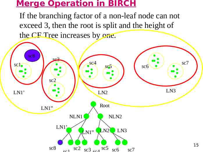
Merge Operation in BIRCH If the branching factor of a non-leaf node can not exceed 3, then the root is split and the height of the CF Tree increases by one. sc8 sc1 sc3 sc4 sc5 sc7 sc6 sc2 LN1’ LN3 LN2 Root LN1” NLN1 LN1’ sc8 LN1” sc2 sc3 NLN2 LN2 LN3 sc5 sc6 sc7 15
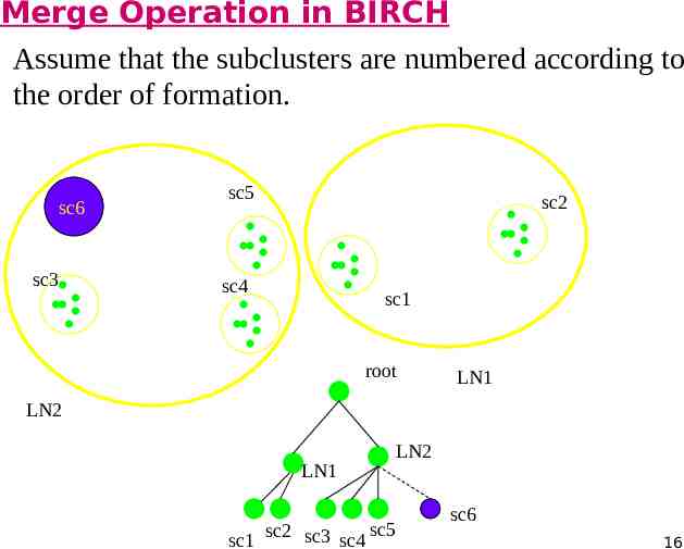
Merge Operation in BIRCH Assume that the subclusters are numbered according to the order of formation. sc6 sc3 sc5 sc2 sc4 sc1 root LN1 LN2 LN1 sc5 sc1 sc2 sc3 sc4 LN2 sc6 16
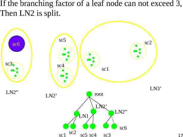
If the branching factor of a leaf node can not exceed 3, Then LN2 is split. sc5 sc6 sc3 LN2” sc2 sc4 sc1 LN3’ root LN2’ LN2’ LN1 sc1 sc2 sc5 sc4 LN2” sc6 sc3 17
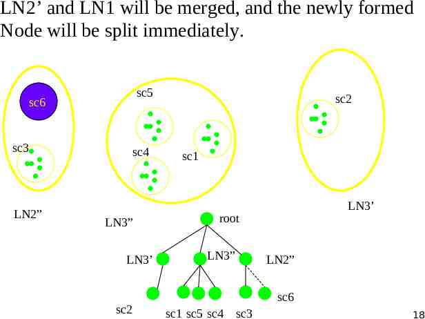
LN2’ and LN1 will be merged, and the newly formed Node will be split immediately. sc5 sc6 sc3 LN2” sc4 LN3” LN3’ sc2 sc2 sc1 LN3’ root LN3” LN2” sc6 sc1 sc5 sc4 sc3 18
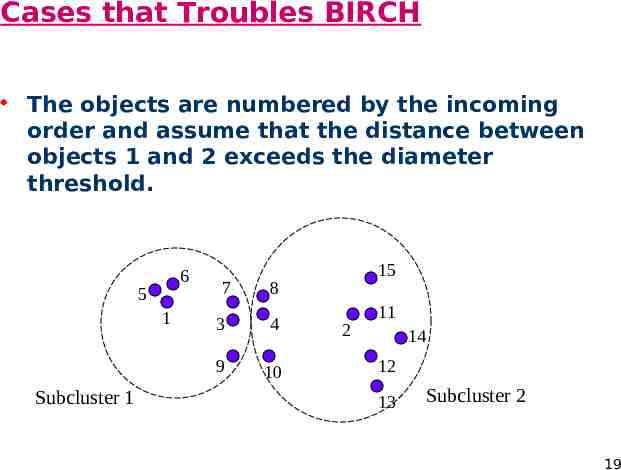
Cases that Troubles BIRCH The objects are numbered by the incoming order and assume that the distance between objects 1 and 2 exceeds the diameter threshold. 6 5 1 Subcluster 1 7 15 8 3 4 9 10 2 11 14 12 13 Subcluster 2 19
Order Dependence Incremental clustering algorithm such as BIRCH suffers order dependence. As the previous example demonstrates, the split and merge operations can alleviate order dependence to certain extent. In the example that demonstrates the merge operation, the split and merge operations together improve clustering quality. However, order dependence can not be completely avoided. If no new objects were added to form subcluster 6, then the clustering quality is not satisfactory. 20
Several Issues with the CF Tree No of entries in CFT node limited by page size; thus, node may not correspond to natural cluster Two sub-clusters that should be in one cluster are splitted across nodes Two sub-clusters that should not be in one cluster are kept in same node (dependent on input order and skewness) Sensitive to skewed input order Data point may end in leaf node where it should not have been If data point is inserted twice at different times, may end up in two copies at two distinct leaf nodes 21
BIRCH Phases X Phase: Global clustering Use existing clustering (e.g., AGNES) algorithm on sub-clusters at leaf nodes May treat each sub-cluster as a point (its centroid) and perform clustering on these points Clusters produced closer to data distribution pattern Phase: Cluster refinement Redistribute (re-label) all data points w.r.t. clusters produced by global clustering This phase may be repeated to improve cluster quality 22
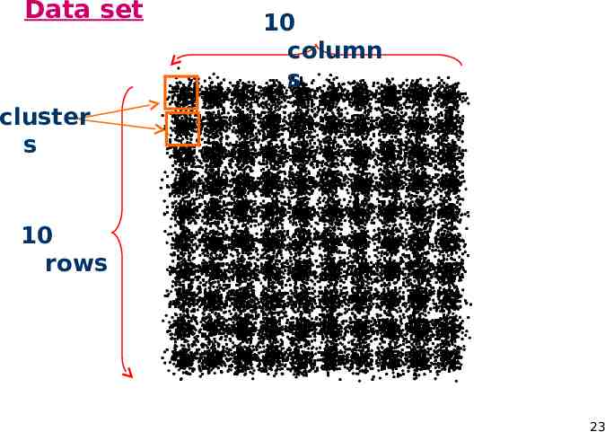
Data set 10 column s cluster s 10 rows 23
BIRCH and CLARANS comparison 24
BIRCH and CLARANS comparison 25
BIRCH and CLARANS comparison 26
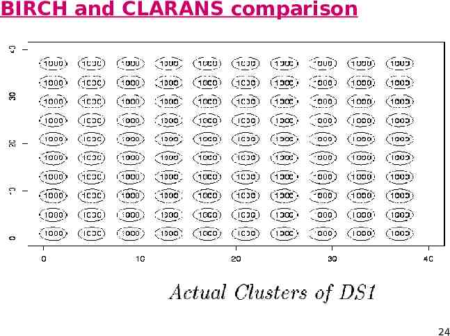
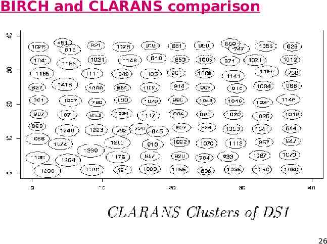
BIRCH and CLARANS comparison Result visualization: Cluster represented as a circle Circle center is centroid; circle radius is cluster radius Number of points in cluster labeled in circle BIRCH results: BIRCH clusters are similar to actual clusters Maximal and average difference between centroids of actual and corresponding BIRCH cluster are 0.17 and 0.07 respectively No of points in BIRCH cluster is no more than 4% different from that of corresponding actual cluster Radii of BIRCH clusters are close to those of actual clusters 27
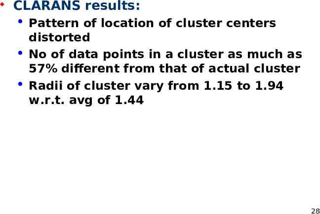
CLARANS results: Pattern of location of cluster centers distorted No of data points in a cluster as much as 57% different from that of actual cluster Radii of cluster vary from 1.15 to 1.94 w.r.t. avg of 1.44 28
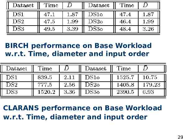
BIRCH performance on Base Workload w.r.t. Time, diameter data set and andinput inputorder order CLARANS performance on Base Workload w.r.t. set and w.r.t. Time, Time, data diameter andinput inputorder order 29
BIRCH and CLARANS comparison Parameters: D: average diameter; smaller means better cluster quality Time: time to cluster datasets (in seconds) Order (‘o’): points in the same cluster are placed together in the input data Results: BIRCH took less than 50 secs to cluster 100,000 data points of each dataset (on an HP 9000 workstation with 80K memory) Ordering of data points also have no impact CLARANS is at least 15 times slower than BIRCH; when data points are ordered, CLARANS performance degrades 30