Introduction to Data Warehousing CPS 196.03 Notes 6
43 Slides675.00 KB
Introduction to Data Warehousing CPS 196.03 Notes 6
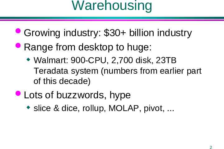
Warehousing Growing industry: 30 billion industry Range from desktop to huge: Walmart: 900-CPU, 2,700 disk, 23TB Teradata system (numbers from earlier part of this decade) Lots of buzzwords, hype slice & dice, rollup, MOLAP, pivot, . 2
Outline What is a data warehouse? Why a warehouse? Models & operations Implementing a warehouse 3
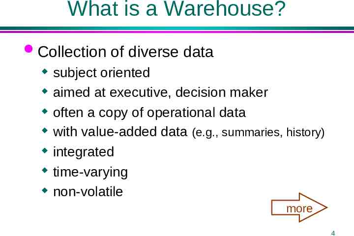
What is a Warehouse? Collection of diverse data subject oriented aimed at executive, decision maker often a copy of operational data with value-added data (e.g., summaries, history) integrated time-varying non-volatile more 4
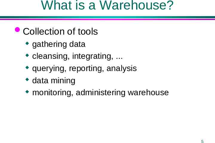
What is a Warehouse? Collection of tools gathering data cleansing, integrating, . querying, reporting, analysis data mining monitoring, administering warehouse 5
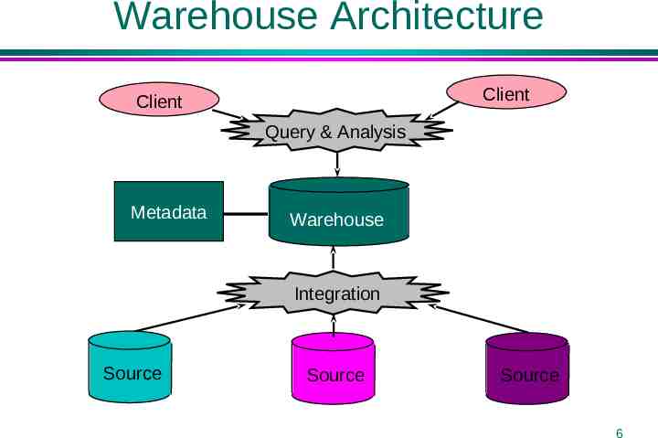
Warehouse Architecture Client Client Query & Analysis Metadata Warehouse Integration Source Source Source 6
Motivating Examples Forecasting Comparing performance of units Monitoring, detecting fraud Visualization 7
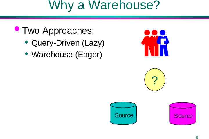
Why a Warehouse? Two Approaches: Query-Driven (Lazy) Warehouse (Eager) ? Source Source 8
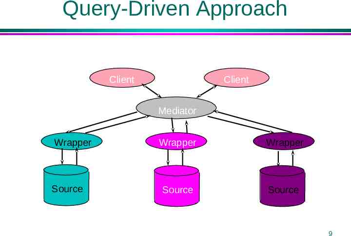
Query-Driven Approach Client Client Mediator Wrapper Source Wrapper Wrapper Source Source 9
Advantages of Warehousing High query performance Queries not visible outside warehouse Local processing at sources unaffected Can operate when sources unavailable Can query data not stored in a DBMS Extra information at warehouse Modify, summarize (store aggregates) Add historical information 10
Advantages of Query-Driven No need to copy data less storage no need to purchase data More up-to-date data Query needs can be unknown Only query interface needed at sources May be less draining on sources 11
OLTP vs. OLAP OLTP: On Line Transaction Processing Describes processing at operational sites OLAP: On Line Analytical Processing Describes processing at warehouse 12
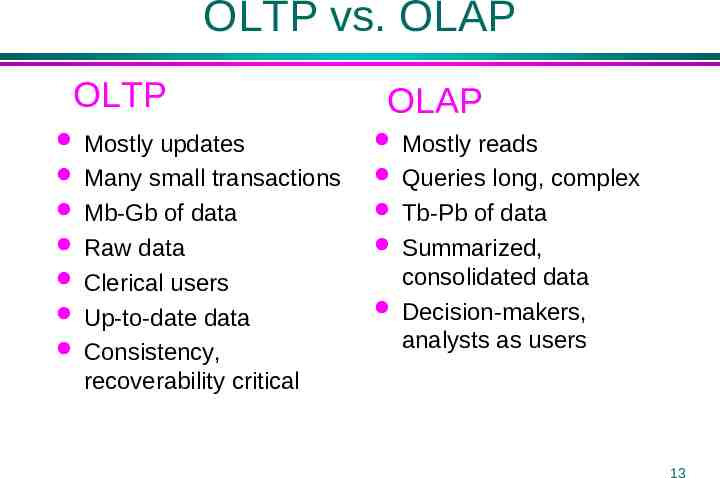
OLTP vs. OLAP OLTP Mostly updates Many small transactions Mb-Gb of data Raw data Clerical users Up-to-date data Consistency, recoverability critical OLAP Mostly reads Queries long, complex Tb-Pb of data Summarized, consolidated data Decision-makers, analysts as users 13
Data Marts Smaller warehouses Spans part of organization e.g., marketing (customers, products, sales) Do not require enterprise-wide consensus but long term integration problems? 14
Warehouse Models & Operators Data Models relations stars & snowflakes cubes Operators slice & dice roll-up, drill down pivoting other 15
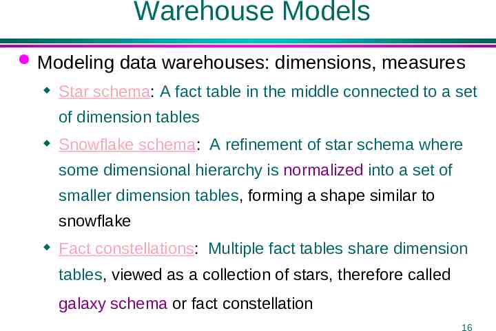
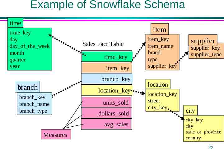
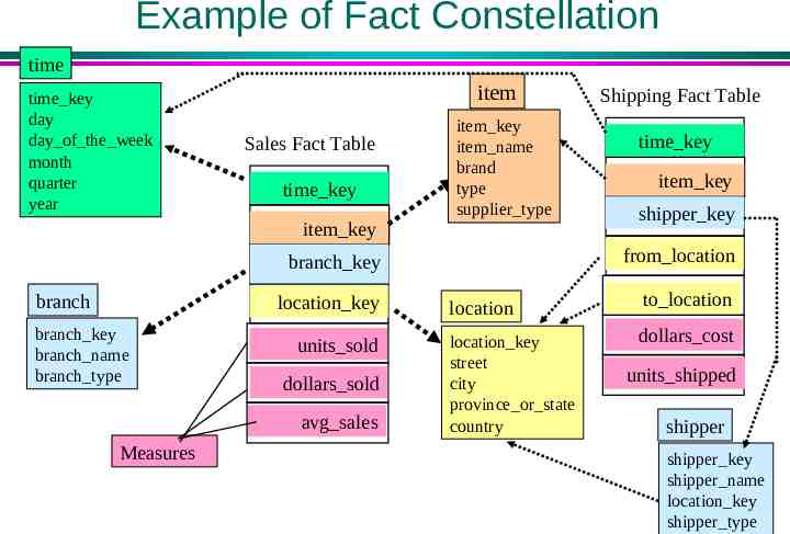
Warehouse Models Modeling data warehouses: dimensions, measures Star schema: A fact table in the middle connected to a set of dimension tables Snowflake schema: A refinement of star schema where some dimensional hierarchy is normalized into a set of smaller dimension tables, forming a shape similar to snowflake Fact constellations: Multiple fact tables share dimension tables, viewed as a collection of stars, therefore called galaxy schema or fact constellation 16
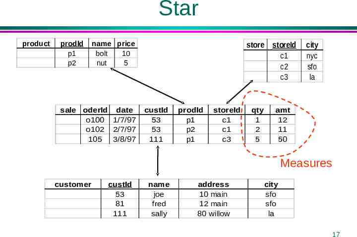
Star product prodId p1 p2 name price bolt 10 nut 5 sale oderId date o100 1/7/97 o102 2/7/97 105 3/8/97 store custId 53 53 111 prodId p1 p2 p1 storeId c1 c1 c3 qty 1 2 5 storeId c1 c2 c3 city nyc sfo la amt 12 11 50 Measures customer custId 53 81 111 name joe fred sally address 10 main 12 main 80 willow city sfo sfo la 17
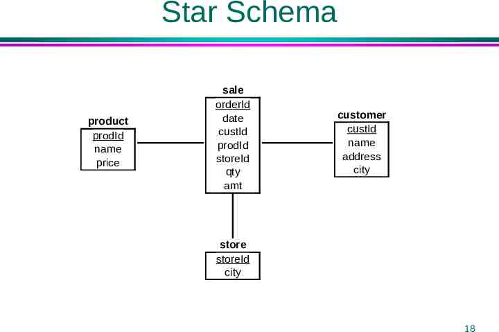
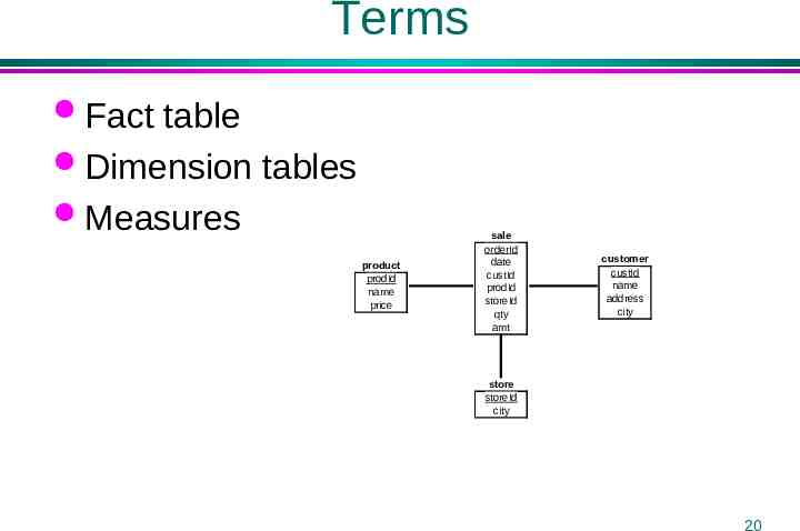
Star Schema product prodId name price sale orderId date custId prodId storeId qty amt customer custId name address city store storeId city 18
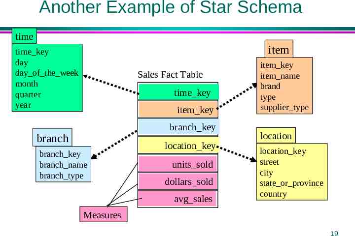
Another Example of Star Schema time item time key day day of the week month quarter year Sales Fact Table time key item key branch key branch branch key branch name branch type location key units sold dollars sold avg sales item key item name brand type supplier type location location key street city state or province country Measures 19
Terms Fact table Dimension tables Measures product prodId name price sale orderId date custId prodId storeId qty amt customer custId name address city store storeId city 20
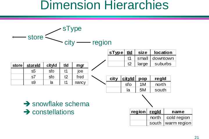
Dimension Hierarchies sType store store storeId s5 s7 s9 city cityId sfo sfo la tId t1 t2 t1 mgr joe fred nancy snowflake schema constellations region sType tId t1 t2 city size small large cityId pop sfo 1M la 5M location downtown suburbs regId north south region regId name north cold region south warm region 21
Example of Snowflake Schema time time key day day of the week month quarter year item Sales Fact Table time key item key branch key branch location key branch key branch name branch type units sold dollars sold avg sales Measures item key item name brand type supplier key supplier supplier key supplier type location location key street city key city city key city state or province country 22
Example of Fact Constellation time time key day day of the week month quarter year item Sales Fact Table time key item key item key item name brand type supplier type location key branch key branch name branch type units sold dollars sold avg sales Measures time key item key shipper key from location branch key branch Shipping Fact Table location to location location key street city province or state country dollars cost units shipped shipper shipper key shipper name location key 23 shipper type
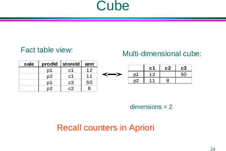
Cube Fact table view: sale prodId p1 p2 p1 p2 storeId c1 c1 c3 c2 Multi-dimensional cube: amt 12 11 50 8 p1 p2 c1 12 11 c2 c3 50 8 dimensions 2 Recall counters in Apriori 24
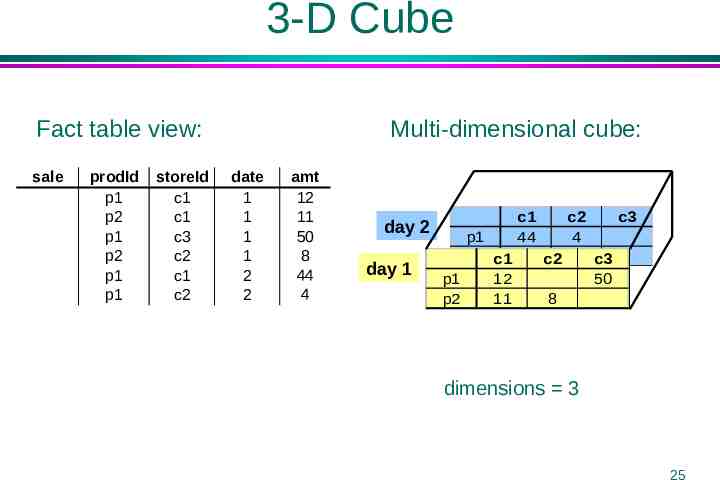
3-D Cube Fact table view: sale prodId p1 p2 p1 p2 p1 p1 storeId c1 c1 c3 c2 c1 c2 Multi-dimensional cube: date 1 1 1 1 2 2 amt 12 11 50 8 44 4 day 2 day 1 p1 p2 c1 p1 12 p2 11 c1 44 c2 4 c2 c3 c3 50 8 dimensions 3 25
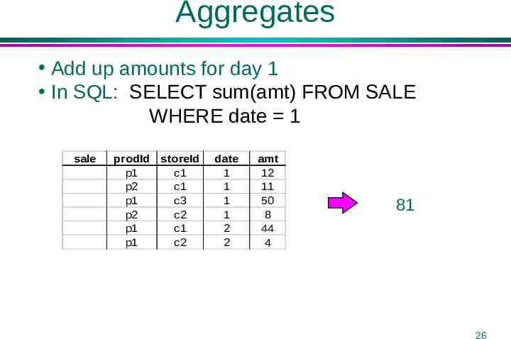
Aggregates Add up amounts for day 1 In SQL: SELECT sum(amt) FROM SALE WHERE date 1 sale prodId p1 p2 p1 p2 p1 p1 storeId c1 c1 c3 c2 c1 c2 date 1 1 1 1 2 2 amt 12 11 50 8 44 4 81 26
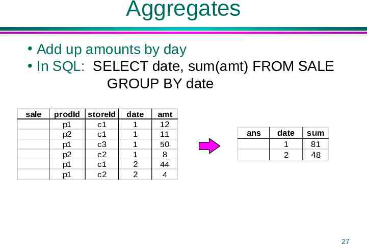
Aggregates Add up amounts by day In SQL: SELECT date, sum(amt) FROM SALE GROUP BY date sale prodId p1 p2 p1 p2 p1 p1 storeId c1 c1 c3 c2 c1 c2 date 1 1 1 1 2 2 amt 12 11 50 8 44 4 ans date 1 2 sum 81 48 27
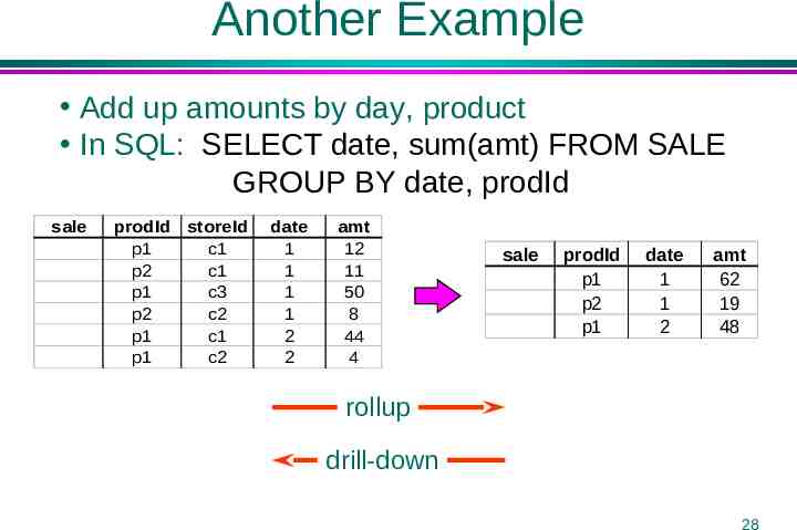
Another Example Add up amounts by day, product In SQL: SELECT date, sum(amt) FROM SALE GROUP BY date, prodId sale prodId storeId p1 c1 p2 c1 p1 c3 p2 c2 p1 c1 p1 c2 date 1 1 1 1 2 2 amt 12 11 50 8 44 4 sale prodId p1 p2 p1 date 1 1 2 amt 62 19 48 rollup drill-down 28
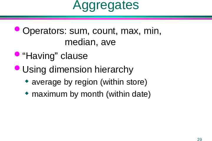
Aggregates Operators: sum, count, max, min, median, ave “Having” clause Using dimension hierarchy average by region (within store) maximum by month (within date) 29
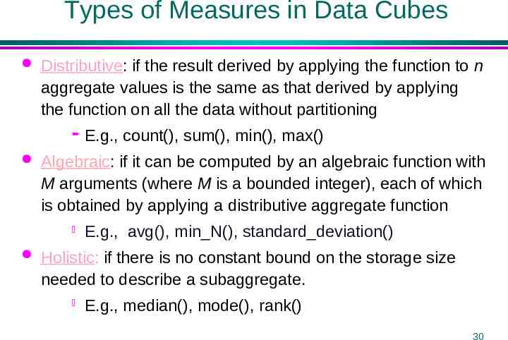
Types of Measures in Data Cubes Distributive: if the result derived by applying the function to n aggregate values is the same as that derived by applying the function on all the data without partitioning Algebraic: if it can be computed by an algebraic function with M arguments (where M is a bounded integer), each of which is obtained by applying a distributive aggregate function E.g., count(), sum(), min(), max() E.g., avg(), min N(), standard deviation() Holistic: if there is no constant bound on the storage size needed to describe a subaggregate. E.g., median(), mode(), rank() 30
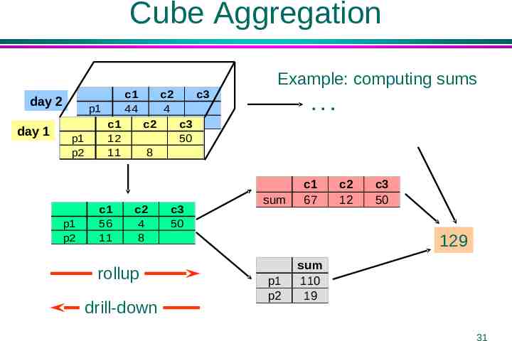
Cube Aggregation day 2 day 1 p1 p2 c1 p1 12 p2 11 p1 p2 c1 56 11 c1 44 c2 4 c2 c3 Example: computing sums . c3 50 8 c2 4 8 rollup drill-down c3 50 sum c1 67 c2 12 c3 50 129 p1 p2 sum 110 19 31
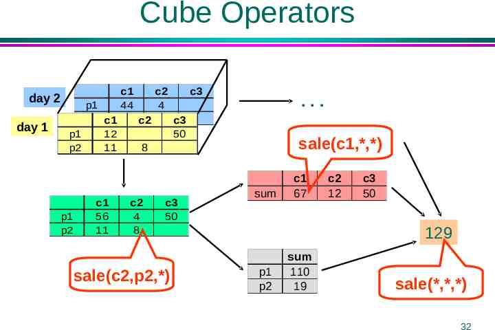
Cube Operators day 2 day 1 p1 p2 c1 p1 12 p2 11 p1 p2 c1 56 11 c1 44 c2 4 c2 c3 . c3 50 sale(c1,*,*) 8 c2 4 8 c3 50 sale(c2,p2,*) sum c1 67 c2 12 c3 50 129 p1 p2 sum 110 19 sale(*,*,*) 32
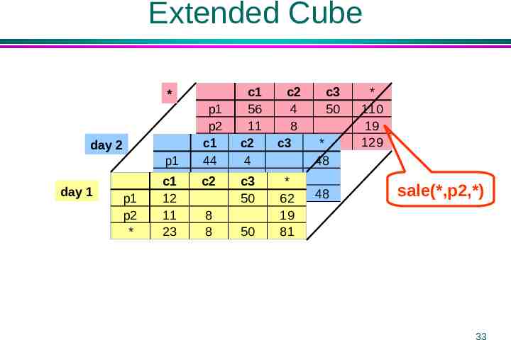
Extended Cube c2 4 8 c312 p1 p2 c1 * 12 p1 p2 c1* 44 c1 56 11 c267 4 c2 44 c3 4 50 11 23 8 8 50 * 62 19 81 * day 2 day 1 p1 p2 * c3 50 * 50 48 48 * 110 19 129 sale(*,p2,*) 33
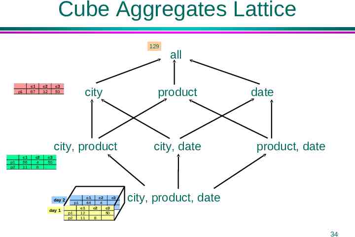
Cube Aggregates Lattice 129 c1 67 p1 c2 12 c3 50 city city, product p1 p2 c1 56 11 c2 4 8 all product city, date date product, date c3 50 day 2 day 1 c1 c2 c3 p1 44 4 p2 c1 c2 c3 p1 12 50 p2 11 8 city, product, date 34
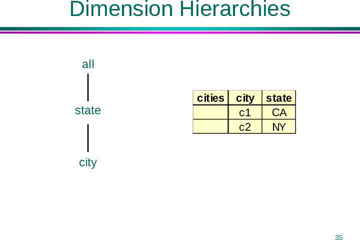
Dimension Hierarchies all state cities city c1 c2 state CA NY city 35
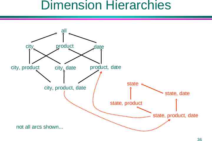
Dimension Hierarchies all city city, product product city, date city, product, date date product, date state state, date state, product state, product, date not all arcs shown. 36
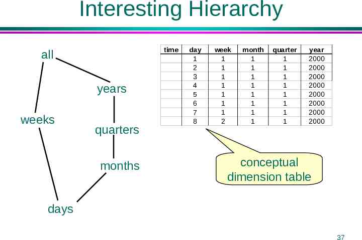
Interesting Hierarchy time all years weeks quarters months day 1 2 3 4 5 6 7 8 week 1 1 1 1 1 1 1 2 month 1 1 1 1 1 1 1 1 quarter 1 1 1 1 1 1 1 1 year 2000 2000 2000 2000 2000 2000 2000 2000 conceptual dimension table days 37
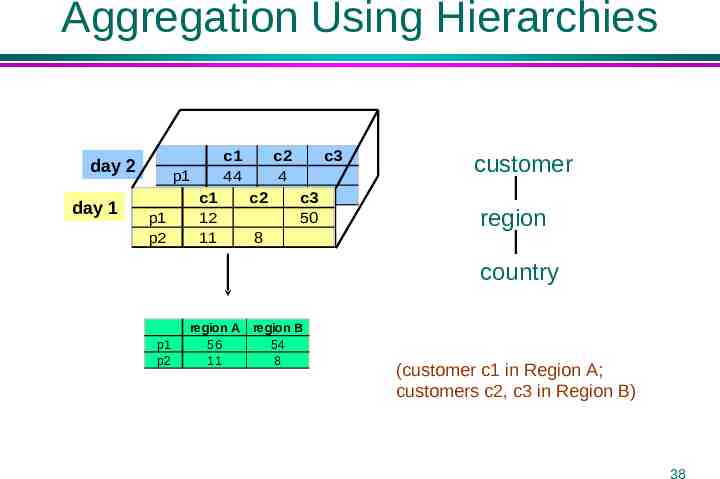
Aggregation Using Hierarchies day 2 day 1 p1 p2 c1 p1 12 p2 11 c1 44 c2 4 c2 c3 c3 50 8 customer region country p1 p2 region A region B 56 54 11 8 (customer c1 in Region A; customers c2, c3 in Region B) 38
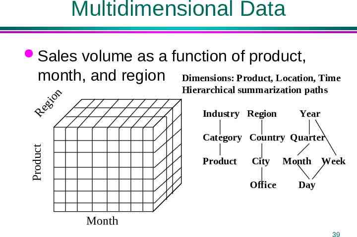
Multidimensional Data Sales volume as a function of product, month, and region Dimensions: Product, Location, Time Hierarchical summarization paths Re gi on Industry Region Year Product Category Country Quarter Product City Office Month Week Day Month 39
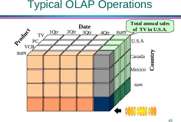
TV PC VCR sum 1Qtr 2Qtr Date 3Qtr 4Qtr sum Total annual sales of TV in U.S.A. U.S.A Canada Mexico Country Pr od uc t Typical OLAP Operations sum 40
Typical OLAP Operations Roll up (drill-up): summarize data by climbing up hierarchy or by dimension reduction Drill down (roll down): reverse of roll-up from higher level summary to lower level summary or detailed data, or introducing new dimensions Slice and dice: project and select Pivot (rotate): reorient the cube, visualization, 3D to series of 2D planes Other operations drill across: involving (across) more than one fact table drill through: through the bottom level of the cube to its backend relational tables (using SQL) 41
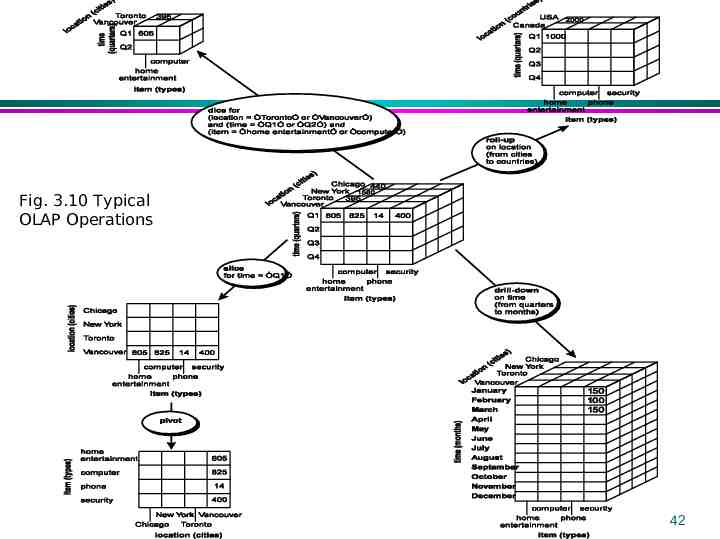
Fig. 3.10 Typical OLAP Operations 42
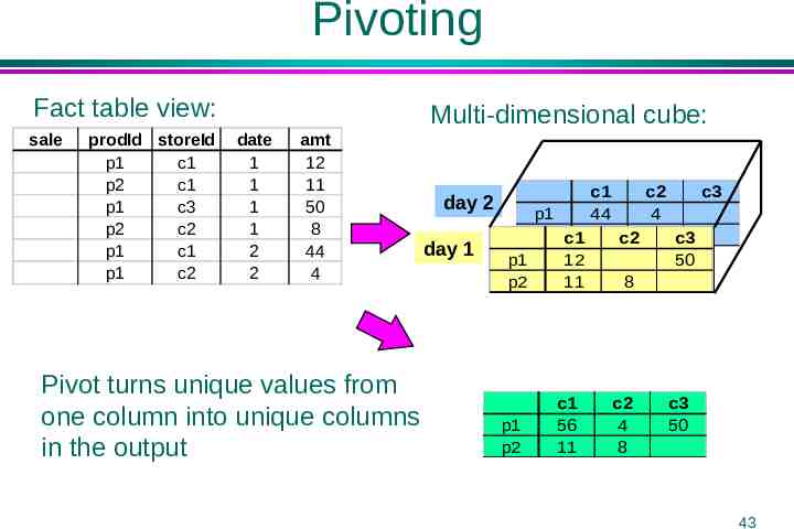
Pivoting Fact table view: sale prodId storeId p1 c1 p2 c1 p1 c3 p2 c2 p1 c1 p1 c2 Multi-dimensional cube: date 1 1 1 1 2 2 amt 12 11 50 8 44 4 Pivot turns unique values from one column into unique columns in the output day 2 day 1 p1 p2 c1 p1 12 p2 11 p1 p2 c1 56 11 c1 44 c2 4 c2 c3 c3 50 8 c2 4 8 c3 50 43