AP Statistics: Chapter 18 Sampling Distribution Models
26 Slides864.00 KB
AP Statistics: Chapter 18 Sampling Distribution Models
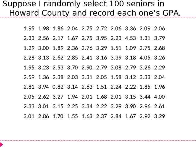
Suppose I randomly select 100 seniors in Howard County and record each one’s GPA. 1.95 1.98 1.86 2.04 2.75 2.72 2.06 3.36 2.09 2.06 2.33 2.56 2.17 1.67 2.75 3.95 2.23 4.53 1.31 3.79 1.29 3.00 1.89 2.36 2.76 3.29 1.51 1.09 2.75 2.68 2.28 3.13 2.62 2.85 2.41 3.16 3.39 3.18 4.05 3.26 1.95 3.23 2.53 3.70 2.90 2.79 3.08 2.79 3.26 2.29 2.59 1.36 2.38 2.03 3.31 2.05 1.58 3.12 3.33 2.04 2.81 3.94 0.82 3.14 2.63 1.51 2.24 2.22 1.85 1.96 2.05 2.62 3.27 1.94 2.01 1.68 2.01 3.15 3.44 4.00 2.33 3.01 3.15 2.25 3.34 2.22 3.29 3.90 2.96 2.61 3.01 2.86 1.70 1.55 1.63 2.37 2.84 1.67 2.92 3.29
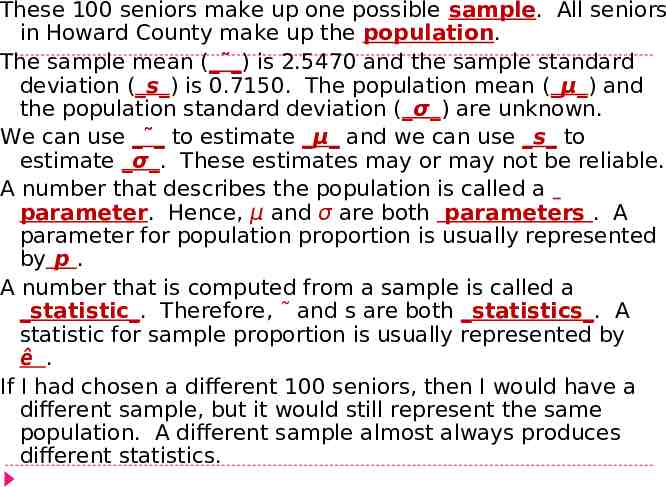
These 100 seniors make up one possible sample. All seniors in Howard County make up the population. The sample mean ( ) is 2.5470 and the sample standard deviation ( s ) is 0.7150. The population mean ( μ ) and the population standard deviation ( σ ) are unknown. We can use to estimate μ and we can use s to estimate σ . These estimates may or may not be reliable. A number that describes the population is called a parameter. Hence, μ and σ are both parameters . A parameter for population proportion is usually represented by p . A number that is computed from a sample is called a statistic . Therefore, and s are both statistics . A statistic for sample proportion is usually represented by ê . If I had chosen a different 100 seniors, then I would have a different sample, but it would still represent the same population. A different sample almost always produces different statistics.
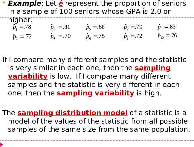
Example: Let ê represent the proportion of seniors in a sample of 100 seniors whose GPA is 2.0 or higher. pˆ1 .78 pˆ 2 .72 pˆ 3 .81 pˆ 4 .70 pˆ 5 .68 pˆ 6 .75 pˆ 7 .79 pˆ 8 .72 pˆ 9 .83 pˆ10 .76 If I compare many different samples and the statistic is very similar in each one, then the sampling variability is low. If I compare many different samples and the statistic is very different in each one, then the sampling variability is high. The sampling distribution model of a statistic is a model of the values of the statistic from all possible samples of the same size from the same population.
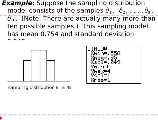
Example: Suppose the sampling distribution model consists of the samples ê1, ê2,.,ê9, ê10. (Note: There are actually many more than ten possible samples.) This sampling model has mean 0.754 and standard deviation 0.049. sampling distribution Ë 4s
The statistic used to estimate a parameter is unbiased if the mean of its sampling distribution model is equal to the true value of the parameter being estimated. Example: Since the mean of the sampling model is 0.754, then ê is an unbiased estimator of p if the true value of p (the proportion of all seniors in Howard County with a GPA of 2.0 or higher) equals 0.754. A statistic can be unbiased and still have high variability. To avoid this, increase the size of the sample. Larger samples give smaller spread.
Sample Proportions: The parameter p is the population proportion. In practice, this value is always unknown. (If we know the population proportion, then there is no need for a sample.) The statistic ê is the sample proportion. We use ê to estimate the value of p . The value of the statistic ê changes as the sample changes. How can we describe the sampling model for ê ? 1. shape? 2. center? 3. spread?
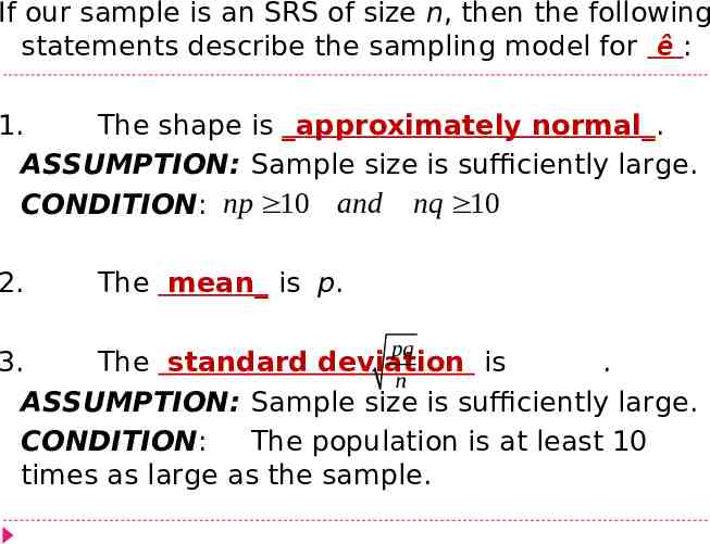
If our sample is an SRS of size n, then the following statements describe the sampling model for ê : 1. The shape is approximately normal . ASSUMPTION: Sample size is sufficiently large. CONDITION: np 10 and nq 10 2. The mean is p. pq 3. The standard deviation is . n ASSUMPTION: Sample size is sufficiently large. CONDITION: The population is at least 10 times as large as the sample.
If we have categorical data, then we must use sample proportions to construct a sampling model. Example: Suppose we want to know how many seniors in Maryland plan to attend college. We want to know how many seniors would answer, “YES” to the question, “Do you plan to attend college?” These responses are categorical .
So p (our parameter) is the proportion of all seniors Maryland who plan to attend college. Let ê (our statistic) be the proportion of Maryland students in an SRS of size 100 who plan to attend college. To calculate the value of ê , we divide the number of “Yes” responses in our sample by the total number of students in the sample.
If I graph the values of ê for all possible samples of size 100, then I have constructed a sampling distribution model for the sampling proportions of size 100 . What will the sampling model look like? It will be approximately normal . In fact, the larger my sample size, the closer it will be to a normal model. It can never be perfectly normal, because our data is discrete, and normal distributions are continuous.
So how large is large enough to ensure that the sampling model is close to normal? Both np and nq should be at least 10 in order for normal approximations to be useful. Furthermore The mean of the sampling model will equal the true population proportion, p . And The standard deviation (if thepqpopulation is at least 10 times as large as the n sample) will be .
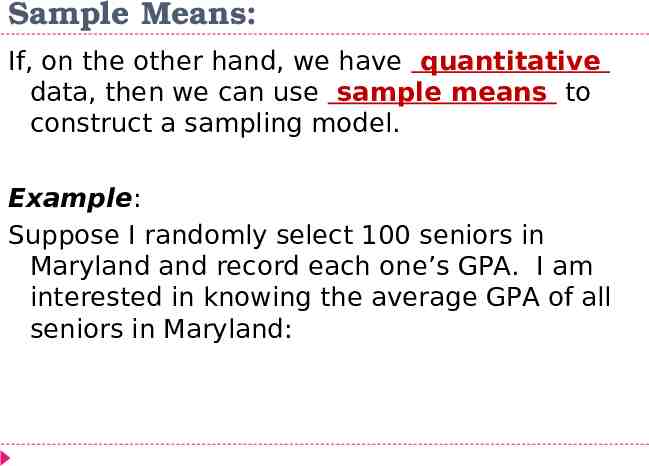
Sample Means: If, on the other hand, we have quantitative data, then we can use sample means to construct a sampling model. Example: Suppose I randomly select 100 seniors in Maryland and record each one’s GPA. I am interested in knowing the average GPA of all seniors in Maryland:
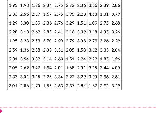
1.95 1.98 1.86 2.04 2.75 2.72 2.06 3.36 2.09 2.06 2.33 2.56 2.17 1.67 2.75 3.95 2.23 4.53 1.31 3.79 1.29 3.00 1.89 2.36 2.76 3.29 1.51 1.09 2.75 2.68 2.28 3.13 2.62 2.85 2.41 3.16 3.39 3.18 4.05 3.26 1.95 3.23 2.53 3.70 2.90 2.79 3.08 2.79 3.26 2.29 2.59 1.36 2.38 2.03 3.31 2.05 1.58 3.12 3.33 2.04 2.81 3.94 0.82 3.14 2.63 1.51 2.24 2.22 1.85 1.96 2.05 2.62 3.27 1.94 2.01 1.68 2.01 3.15 3.44 4.00 2.33 3.01 3.15 2.25 3.34 2.22 3.29 3.90 2.96 2.61 3.01 2.86 1.70 1.55 1.63 2.37 2.84 1.67 2.92 3.29
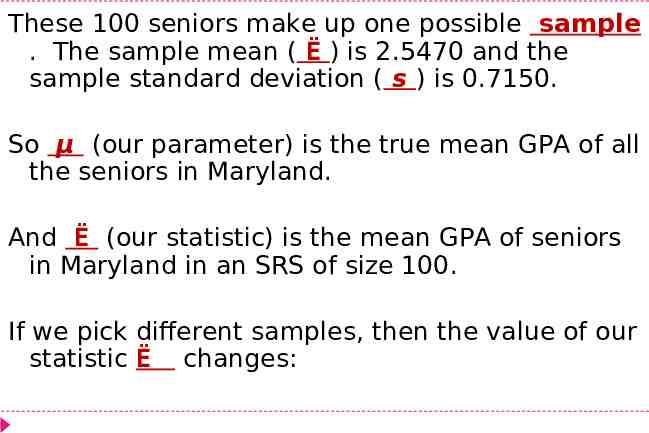
These 100 seniors make up one possible sample . The sample mean ( Ë ) is 2.5470 and the sample standard deviation ( s ) is 0.7150. So μ (our parameter) is the true mean GPA of all the seniors in Maryland. And Ë (our statistic) is the mean GPA of seniors in Maryland in an SRS of size 100. If we pick different samples, then the value of our statistic Ë changes:
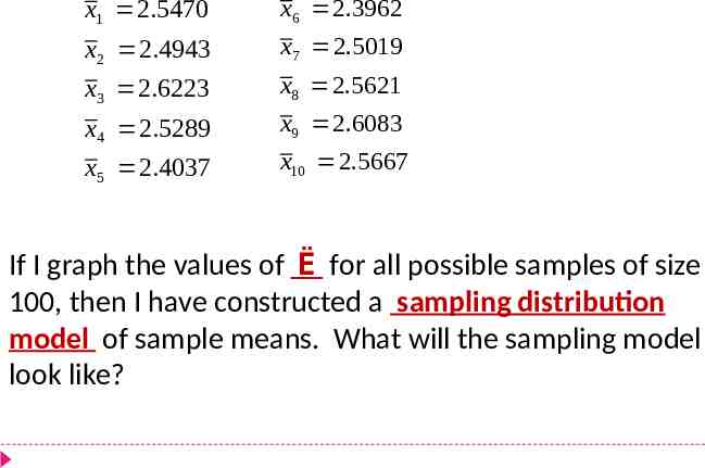
x1 2.5470 x6 2.3962 x 2 2.4943 x7 2.5019 x3 2.6223 x8 2.5621 x 4 2.5289 x9 2.6083 x5 2.4037 x10 2.5667 If I graph the values of Ë for all possible samples of size 100, then I have constructed a sampling distribution model of sample means. What will the sampling model look like?
Remember that each Ë value is a mean. Means are less variable than individual observations because if we are looking only at means, then we don’t see any extreme values, only average values. We won’t see GPA’s that are very low or very high, only average GPA’s. The larger the sample size, the less variation we will see in the values of Ë . So the standard deviation decreases as the sample size increases.
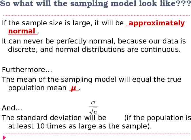
So what will the sampling model look like? If the sample size is large, it will be approximately normal . It can never be perfectly normal, because our data is discrete, and normal distributions are continuous. Furthermore The mean of the sampling model will equal the true population mean μ . n And The standard deviation will be (if the population is at least 10 times as large as the sample).
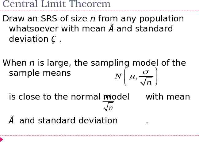
Central Limit Theorem Draw an SRS of size n from any population whatsoever with mean à and standard deviation Ç . When n is large, the sampling model of the sample means N , is close to the normal model n with mean n à and standard deviation .
Law of Large Numbers Draw observations at random from any population with mean Ã. As the number of observations increases, the sample mean Ë gets closer and closer to Ã.
Use the 68-95-99.7 Rule to answer the following. Be sure to check the conditions first. 1) Of all the cars on the interstate, 80% exceed the speed limit. What proportion of speeders might we see among the next 50 cars?
Use the 68-95-99.7 Rule to answer the following. Be sure to check the conditions first. 2) We don’t know it, but 52% of voters plan to vote “Yes” on the upcoming school budget. We poll a random sample of 300 voters. What might the percentage of yes-voters appear to be in our poll?
Use the sampling models to calculate some probabilities. 3) “Groovy” M&M’s are supposed to make up 30% of the candies sold. In a large bag of 250 M&M’s, what is the probability that we get at least 25% groovy candies?
Use the Central Limit Theorem (CLT) together with the 68-95-99.7 Rule and the normal percentiles to answer the following: 4) SAT scores follow a normal model and should have a mean of 500 and a standard deviation of100. What are the mean and standard deviation of the distribution of all random samples of 20 students?
Use the Central Limit Theorem (CLT) together with the 68-95-99.7 Rule and the normal percentiles to answer the following: 5) Speeds of cars on a highway have mean 52 mph and standard deviation 6 mph, and are likely to be skewed to the right (a few very fast drivers). Describe what we might see in random samples of 50 cars.
Use the Central Limit Theorem (CLT) together with the 68-95-99.7 Rule and the normal percentiles to answer the following: 6) At birth, babies average 7.8 pounds, with a standard deviation of 2.1 pounds. A random sample of 34 babies born to mothers living near a large factory that may be polluting the air and water shows a mean birthweight of only 7.2 pounds. Is that unusually low?