A philosophical basis for Valuation Many investors believe that


87 Slides403.50 KB
A philosophical basis for Valuation Many investors believe that the pursuit of 'true value' based upon financial fundamentals is a fruitless one in markets where prices often seem to have little to do with value. There have always been investors in financial markets who have argued that market prices are determined by the perceptions (and misperceptions) of buyers and sellers, and not by anything as prosaic as cashflows or earnings. Perceptions matter, but they cannot be all that matter. Asset prices cannot be justified by merely using the “bigger fool” theory.
Misconceptions about Valuation Myth 1: A valuation is an objective search for “true” value – Truth 1.1: All valuations are biased. The only questions are how much and in which direction. – Truth 1.2: The direction and magnitude of the bias in your valuation is directly proportional to who pays you and how much you are paid. Myth 2.: A good valuation provides a precise estimate of value – Truth 2.1: There are no precise valuations – Truth 2.2: The payoff to valuation is greatest when valuation is least precise. Myth 3: . The more quantitative a model, the better the valuation – Truth 3.1: One’s understanding of a valuation model is inversely proportional to the number of inputs required for the model. – Truth 3.2: Simpler valuation models do much better than complex ones.
Fundamental Approaches to Valuation Discounted cashflow valuation: Relates the value of an asset to the present value of expected future cashflows on that asset. Relative valuation: Estimates the value of an asset by looking at the pricing of 'comparable' assets relative to a common variable like earnings, cashflows, book value or sales. Contingent claim valuation: Uses option pricing models to measure the value of assets that share option characteristics.
Basis for all valuation approaches The use of valuation models in investment decisions (i.e., in decisions on which assets are under valued and which are over valued) are based upon – a perception that markets are inefficient and make mistakes in assessing value – an assumption about how and when these inefficiencies will get corrected In an efficient market, the market price is the best estimate of value. The purpose of any valuation model is then the justification of this value.
Efficient Market Hypothesis (EMH) Definition 1: A market is said to be efficient with respect to some information set, It, if it is impossible to make economic profits on the basis of information set It. – Economic profits: Profits after adjusting for risk and transaction costs (such as, brokerage fees, investment advisory fees). – Economic profits Actual return - Expected return - Transaction costs – Expected Return: CAPM provides one estimate of expected return. Other estimates: Arbitrage Pricing Theory, Historical Industry Returns.
EMH continued: Models of Expected Returns – CAPM: Expected return on stock i Riskfree rate (Beta of i with respect to Market)*(Expected return on Market - Riskfree rate) – APT: Expected return on stock i Riskfree rate (Beta of i with respect to Factor 1)*(Expected return on Factor 1 - Riskfree rate) (Beta of i with respect to Factor 2)*(Expected return on Factor 2 - Riskfree rate) .
EMH continued Models of Expected Returns – Historical Industry Returns: Expected Return on stock i Average historical return of other firms in the same industry as company i.
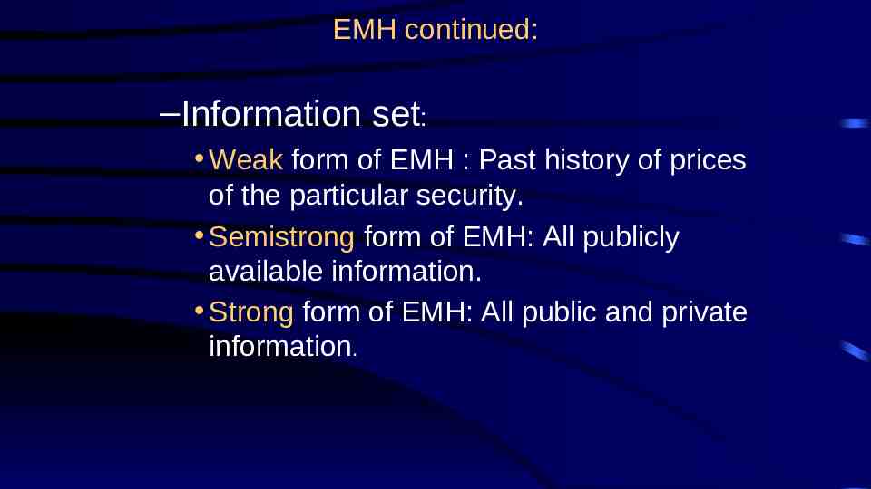
EMH continued: –Information set: Weak form of EMH : Past history of prices of the particular security. Semistrong form of EMH: All publicly available information. Strong form of EMH: All public and private information.
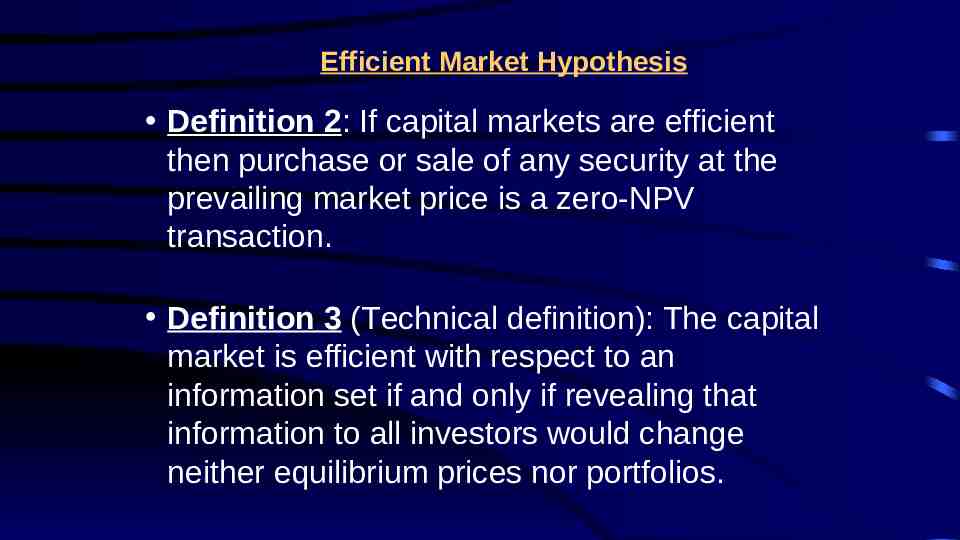
Efficient Market Hypothesis Definition 2: If capital markets are efficient then purchase or sale of any security at the prevailing market price is a zero-NPV transaction. Definition 3 (Technical definition): The capital market is efficient with respect to an information set if and only if revealing that information to all investors would change neither equilibrium prices nor portfolios.
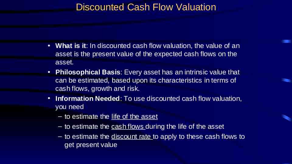
Discounted Cash Flow Valuation What is it: In discounted cash flow valuation, the value of an asset is the present value of the expected cash flows on the asset. Philosophical Basis: Every asset has an intrinsic value that can be estimated, based upon its characteristics in terms of cash flows, growth and risk. Information Needed: To use discounted cash flow valuation, you need – to estimate the life of the asset – to estimate the cash flows during the life of the asset – to estimate the discount rate to apply to these cash flows to get present value
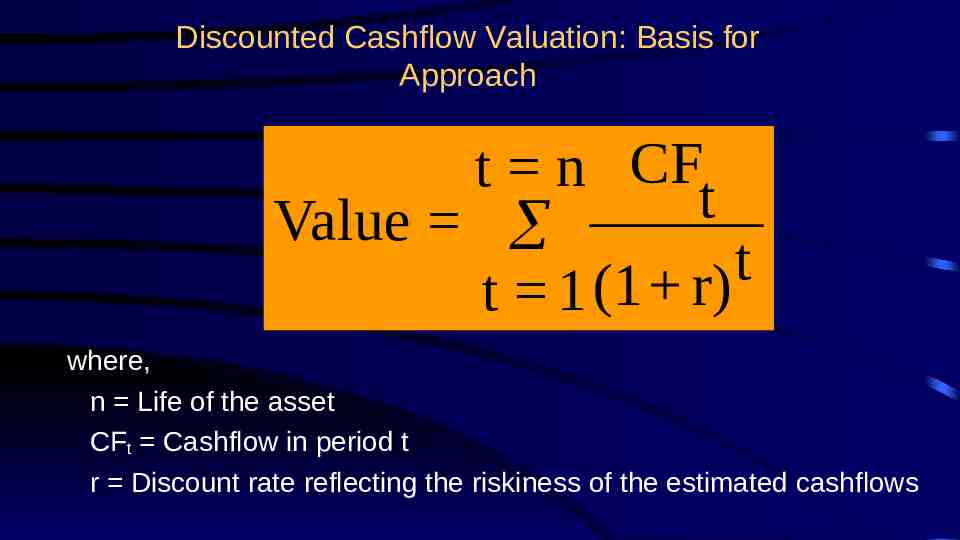
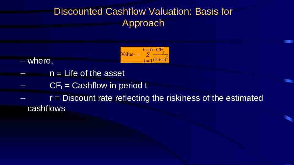
Discounted Cashflow Valuation: Basis for Approach t n CF t Value t t 1 (1 r) where, n Life of the asset CFt Cashflow in period t r Discount rate reflecting the riskiness of the estimated cashflows
Advantages of DCF Valuation Since DCF valuation, done right, is based upon an asset’s fundamentals, it should be less exposed to market moods and perceptions. If good investors buy businesses, rather than stocks (the Warren Buffett adage), discounted cash flow valuation is the right way to think about what you are getting when you buy an asset. DCF valuation forces you to think about the underlying characteristics of the firm, and understand its business. If nothing else, it brings you face to face with the assumptions you are making when you pay a given price for an asset.
Disadvantages of DCF valuation Since it is an attempt to estimate intrinsic value, it requires far more inputs and information than other valuation approaches These inputs and information are not only noisy (and difficult to estimate), but can be manipulated by the savvy analyst to provide the conclusion he or she wants. For example: – An entrepreneur can get a high valuation by overestimating cashflows and/or underestimating discount rates. – A venture capitalist can buy equity from an entrepreneur at a lower price by underestimating cashflows. – An entrepreneur and venture capitalist can get a higher price for their IPO by overestimating cashflows and/or underestimating discount rates.
Disadvantages of DCF valuation In an intrinsic valuation model, there is no guarantee that anything will emerge as under- or over-valued. Thus, it is possible in a DCF valuation model, to find every stock in a market to be over-valued. This can be a problem for – equity research analysts, whose job it is to follow sectors and make recommendations on the most under- and over-valued stocks in that sector – equity portfolio managers, who have to be fully (or close to fully) invested in equities
When DCF Valuation works best This approach is easiest to use for assets (firms) whose – cashflows are currently positive and – can be estimated with some reliability for future periods, and – where a proxy for risk that can be used to obtain discount rates is available. It works best for investors who either – have a long time horizon, allowing the market time to correct its valuation mistakes and for price to revert to “true” value or – are capable of providing the catalyst needed to move price to value, as would be the case if you were an activist investor or a potential acquirer of the whole firm
Relative Valuation What is it?: The value of any asset can be estimated by looking at how the market prices “similar” or ‘comparable” assets. Philosophical Basis: The intrinsic value of an asset is impossible (or close to impossible) to estimate. The value of an asset is whatever the market is willing to pay for it (based upon its characteristics) Information Needed: To do a relative valuation, you need – an identical asset, or a group of comparable or similar assets – a standardized measure of value (in equity, this is obtained by dividing the price by a common variable, such as earnings or book value) – and if the assets are not perfectly comparable, variables to control for the differences Market Inefficiency: Pricing errors made across similar or comparable assets are easier to spot, easier to exploit and are much more quickly corrected.
Advantages of Relative Valuation Relative valuation is much more likely to reflect market perceptions and moods than discounted cash flow valuation. This can be an advantage when it is important that the price reflect these perceptions as is the case when – the objective is to sell a security at that price today (as in the case of an IPO) With relative valuation, there will always be a significant proportion of securities that are under- valued and over-valued. Since portfolio managers are judged based upon how they perform on a relative basis (to the market and other money managers), relative valuation is more tailored to their needs Relative valuation generally requires less information than discounted cash flow valuation (especially when multiples are used as screens)
Disadvantages of Relative Valuation A portfolio that is composed of stocks which are undervalued on a relative basis may still be overvalued, even if the analysts’ judgments are right. It is just less overvalued than other securities in the market. Relative valuation is built on the assumption that markets are correct in the aggregate, but make mistakes on individual securities. To the degree that markets can be over or under valued in the aggregate, relative valuation will fail Relative valuation may require less information in the way in which most analysts and portfolio managers use it. However, this is because implicit assumptions are made about other variables (that would have been required in a discounted cash flow valuation). To the extent that these implicit assumptions are wrong the relative valuation will also be wrong.
Introduction DCF Valuation Relative Valuation Real Option Valuation Conclusion Disadvantages of Relative Valuation Relative valuation may require less information in the way in which most analysts and portfolio managers use it. However, this is because implicit assumptions are made about other variables (that would have been required in a discounted cash flow valuation). To the extent that these implicit assumptions are wrong the relative valuation will also be wrong. 19
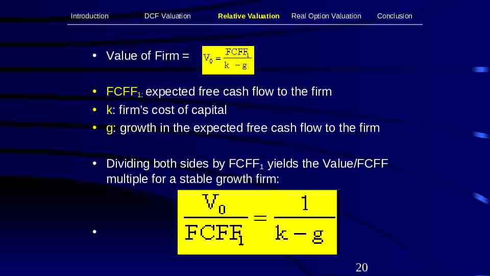
Introduction DCF Valuation Relative Valuation Real Option Valuation Conclusion Value of Firm FCFF1: expected free cash flow to the firm k: firm’s cost of capital g: growth in the expected free cash flow to the firm Dividing both sides by FCFF1 yields the Value/FCFF multiple for a stable growth firm: 20
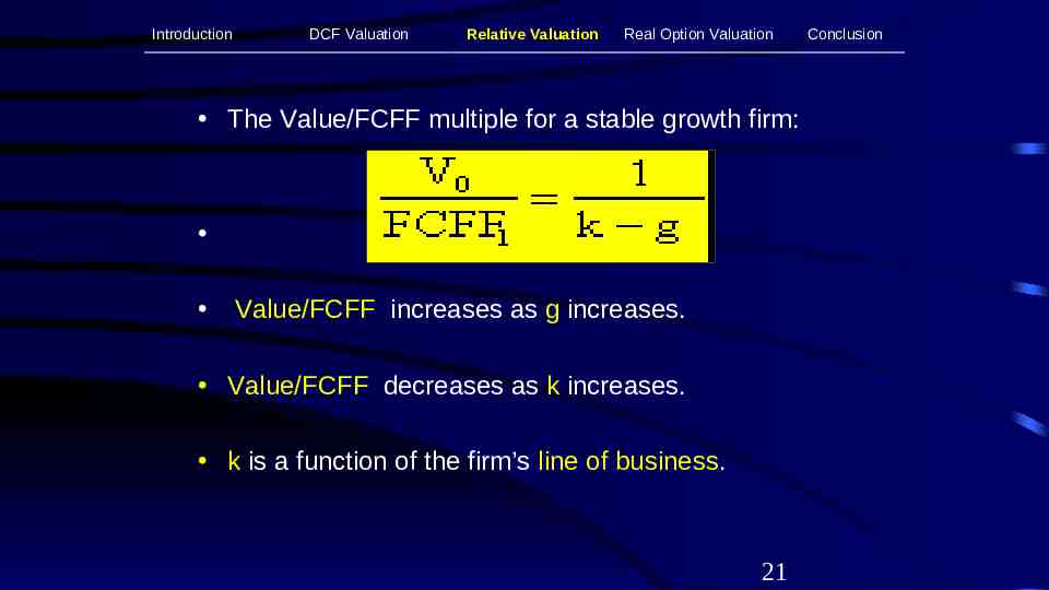
Introduction DCF Valuation Relative Valuation Real Option Valuation The Value/FCFF multiple for a stable growth firm: Value/FCFF increases as g increases. Value/FCFF decreases as k increases. k is a function of the firm’s line of business. 21 Conclusion
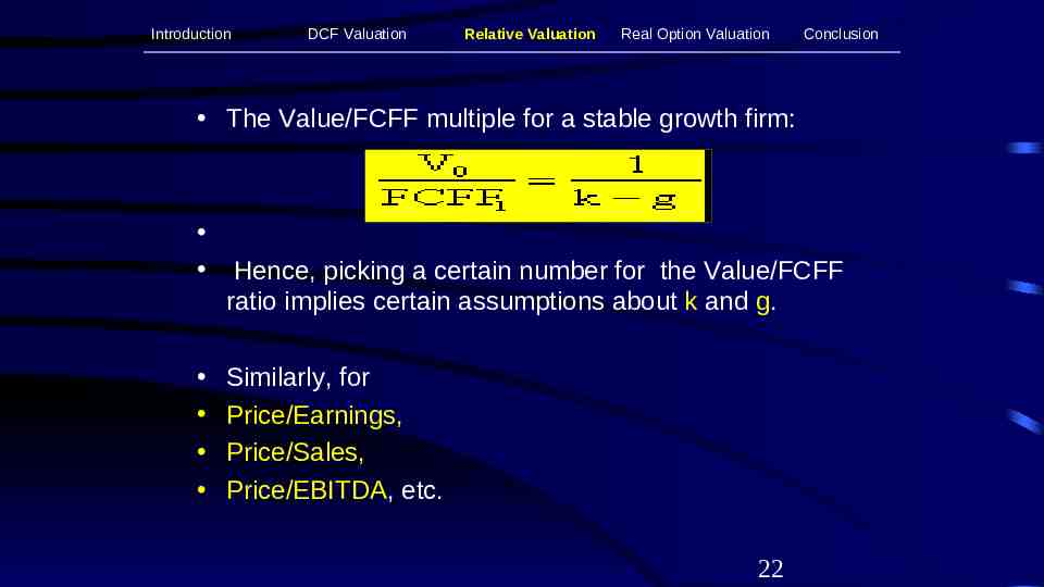
Introduction DCF Valuation Relative Valuation Real Option Valuation Conclusion The Value/FCFF multiple for a stable growth firm: Hence, picking a certain number for the Value/FCFF ratio implies certain assumptions about k and g. Similarly, for Price/Earnings, Price/Sales, Price/EBITDA, etc. 22
When relative valuation works best. This approach is easiest to use when – there are a large number of assets comparable to the one being valued – these assets are priced in a market – there exists some common variable that can be used to standardize the price This approach tends to work best for investors – who have relatively short time horizons – are judged based upon a relative benchmark (the market, other portfolio managers following the same investment style etc.) – can take actions that can take advantage of the relative mispricing; for instance, a portfolio manager specializing in technology stocks can buy the under valued and sell the over valued assets
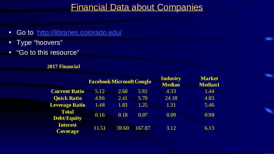
Financial Data about Companies Go to http://libraries.colorado.edu/ Type “hoovers” “Go to this resource” 2017 Financial 5.12 4.96 1.48 2.60 2.41 1.83 5.92 5.70 1.25 Industry Median 4.33 24.18 1.31 0.16 0.18 0.07 0.09 0.98 11.51 59.60 167.87 3.12 6.13 Facebook Microsoft Google Current Ratio Quick Ratio Leverage Ratio Total Debt/Equity Interest Coverage Market Median1 1.44 4.83 5.46
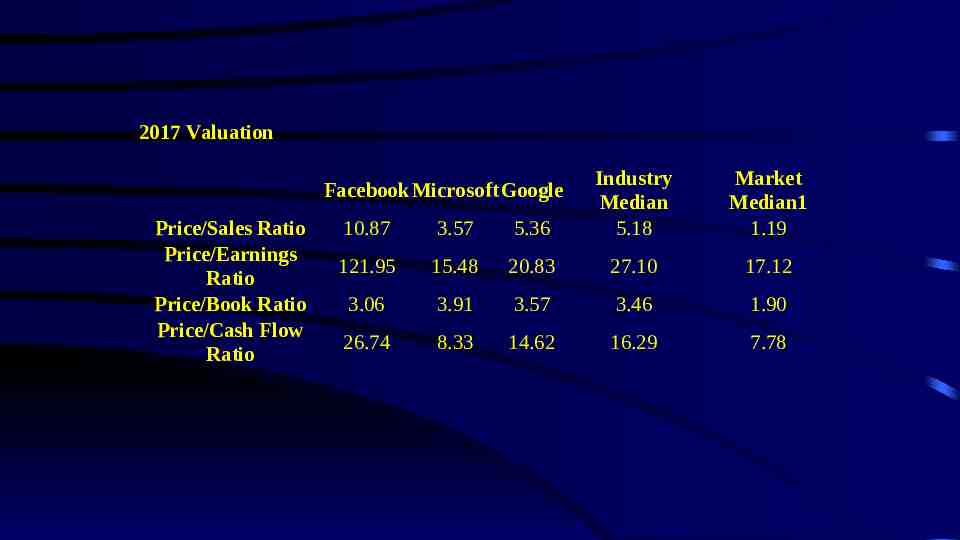
2017 Valuation 10.87 3.57 5.36 Industry Median 5.18 121.95 15.48 20.83 27.10 17.12 3.06 3.91 3.57 3.46 1.90 26.74 8.33 14.62 16.29 7.78 Facebook Microsoft Google Price/Sales Ratio Price/Earnings Ratio Price/Book Ratio Price/Cash Flow Ratio Market Median1 1.19
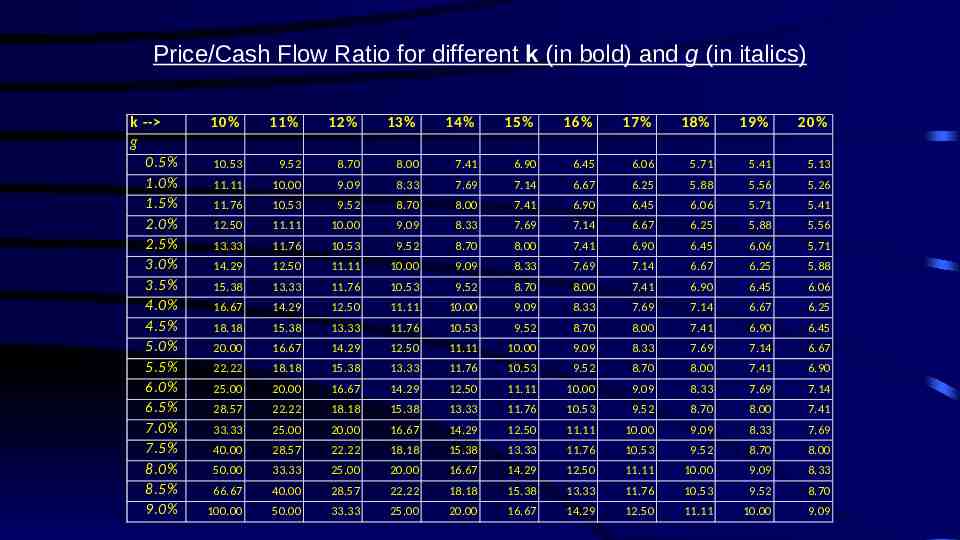
Price/Cash Flow Ratio for different k (in bold) and g (in italics) k -- g 0.5% 1.0% 1.5% 2.0% 2.5% 3.0% 3.5% 4.0% 4.5% 5.0% 5.5% 6.0% 6.5% 7.0% 7.5% 8.0% 8.5% 9.0% 10% 11% 12% 13% 14% 15% 16% 17% 18% 19% 20% 10.53 9.52 8.70 8.00 7.41 6.90 6.45 6.06 5.71 5.41 5.13 11.11 10.00 9.09 8.33 7.69 7.14 6.67 6.25 5.88 5.56 5.26 11.76 10.53 9.52 8.70 8.00 7.41 6.90 6.45 6.06 5.71 5.41 12.50 11.11 10.00 9.09 8.33 7.69 7.14 6.67 6.25 5.88 5.56 13.33 11.76 10.53 9.52 8.70 8.00 7.41 6.90 6.45 6.06 5.71 14.29 12.50 11.11 10.00 9.09 8.33 7.69 7.14 6.67 6.25 5.88 15.38 13.33 11.76 10.53 9.52 8.70 8.00 7.41 6.90 6.45 6.06 16.67 14.29 12.50 11.11 10.00 9.09 8.33 7.69 7.14 6.67 6.25 18.18 15.38 13.33 11.76 10.53 9.52 8.70 8.00 7.41 6.90 6.45 20.00 16.67 14.29 12.50 11.11 10.00 9.09 8.33 7.69 7.14 6.67 22.22 18.18 15.38 13.33 11.76 10.53 9.52 8.70 8.00 7.41 6.90 25.00 20.00 16.67 14.29 12.50 11.11 10.00 9.09 8.33 7.69 7.14 28.57 22.22 18.18 15.38 13.33 11.76 10.53 9.52 8.70 8.00 7.41 33.33 25.00 20.00 16.67 14.29 12.50 11.11 10.00 9.09 8.33 7.69 40.00 28.57 22.22 18.18 15.38 13.33 11.76 10.53 9.52 8.70 8.00 50.00 33.33 25.00 20.00 16.67 14.29 12.50 11.11 10.00 9.09 8.33 66.67 40.00 28.57 22.22 18.18 15.38 13.33 11.76 10.53 9.52 8.70 100.00 50.00 33.33 25.00 20.00 16.67 14.29 12.50 11.11 10.00 9.09
Contingent Claim (Option) Valuation Options have several features – They derive their value from an underlying asset, which has value – The payoff on a call (put) option occurs only if the value of the underlying asset is greater (lesser) than an exercise price that is specified at the time the option is created. If this contingency does not occur, the option is worthless. – They have a fixed life Any security or project that shares these features can be valued as an option.
Direct Examples of Options Listed options, which are options on traded assets, that are issued by, listed on and traded on an option exchange. Warrants, which are call options on traded stocks, that are issued by the company. The proceeds from the warrant issue go to the company, and the warrants are often traded on the market.
Indirect Examples of Options Equity in a deeply troubled firm - a firm with negative earnings and high leverage can be viewed as an option to liquidate that is held by the stockholders of the firm. Viewed as such, it is a call option on the assets of the firm. The reserves owned by natural resource firms can be viewed as call options on the underlying resource, since the firm can decide whether and how much of the resource to extract from the reserve, The patent owned by a firm or an exclusive license issued to a firm can be viewed as an option on the underlying product (project). The firm owns this option for the duration of the patent.
Advantages of Using Option Pricing Models Option pricing models allow us to value assets that we otherwise would not be able to value. For instance, equity in deeply troubled firms and the stock of a small, bio-technology firm (with no revenues and profits) are difficult to value using discounted cash flow approaches or with multiples. They can be valued using option pricing. Option pricing models provide us fresh insights into the drivers of value. In cases where an asset is deriving its value from its option characteristics, for instance, more risk or variability can increase value rather than decrease it.
Disadvantages of Option Pricing Models When real options (which includes the natural resource options and the product patents) are valued, many of the inputs for the option pricing model are difficult to obtain. For instance, projects do not trade and thus getting a current value for a project or a variance may be a daunting task. The option pricing models derive their value from an underlying asset. Thus, to do option pricing, you first need to value the assets. It is therefore an approach that is an addendum to another valuation approach.
Discounted Cash Flow Valuation
Discounted Cashflow Valuation: Basis for Approach t n CF t Value t t 1 (1 r) – where, – n Life of the asset – CFt Cashflow in period t – r Discount rate reflecting the riskiness of the estimated cashflows
Equity Valuation versus Firm Valuation Value just the equity stake in the business Value the entire business, which includes, besides equity, the other claimholders in the firm
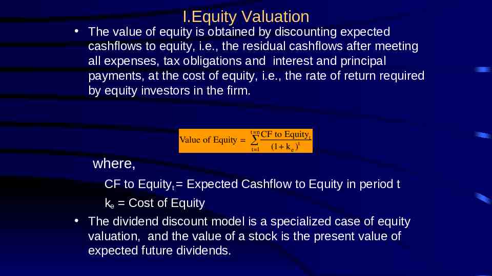
I.Equity Valuation The value of equity is obtained by discounting expected cashflows to equity, i.e., the residual cashflows after meeting all expenses, tax obligations and interest and principal payments, at the cost of equity, i.e., the rate of return required by equity investors in the firm. t n Value of Equity CF to Equityt (1 k )t t 1 e where, CF to Equityt Expected Cashflow to Equity in period t ke Cost of Equity The dividend discount model is a specialized case of equity valuation, and the value of a stock is the present value of expected future dividends.
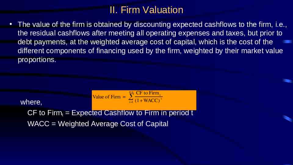
II. Firm Valuation The value of the firm is obtained by discounting expected cashflows to the firm, i.e., the residual cashflows after meeting all operating expenses and taxes, but prior to debt payments, at the weighted average cost of capital, which is the cost of the different components of financing used by the firm, weighted by their market value proportions. t n Value of Firm CF to Firm t t t 1 (1 WACC) where, CF to Firmt Expected Cashflow to Firm in period t WACC Weighted Average Cost of Capital
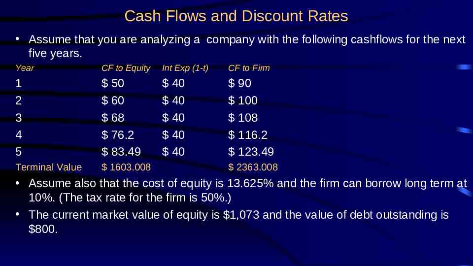
Cash Flows and Discount Rates Assume that you are analyzing a company with the following cashflows for the next five years. Year CF to Equity Int Exp (1-t) CF to Firm 1 2 3 4 5 50 60 68 76.2 83.49 40 40 40 40 40 90 100 108 116.2 123.49 Terminal Value 1603.008 2363.008 Assume also that the cost of equity is 13.625% and the firm can borrow long term at 10%. (The tax rate for the firm is 50%.) The current market value of equity is 1,073 and the value of debt outstanding is 800.
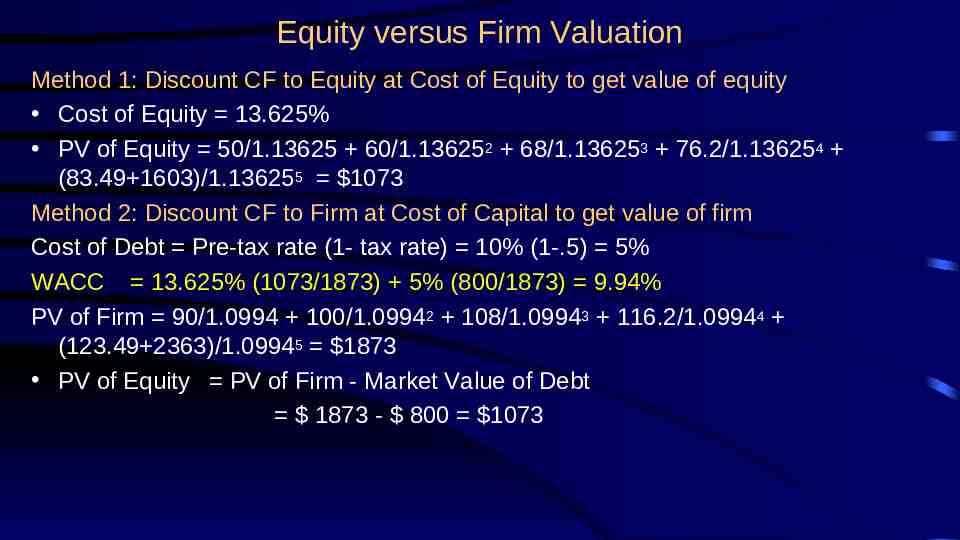
Equity versus Firm Valuation Method 1: Discount CF to Equity at Cost of Equity to get value of equity Cost of Equity 13.625% PV of Equity 50/1.13625 60/1.136252 68/1.136253 76.2/1.136254 (83.49 1603)/1.136255 1073 Method 2: Discount CF to Firm at Cost of Capital to get value of firm Cost of Debt Pre-tax rate (1- tax rate) 10% (1-.5) 5% WACC 13.625% (1073/1873) 5% (800/1873) 9.94% PV of Firm 90/1.0994 100/1.09942 108/1.09943 116.2/1.09944 (123.49 2363)/1.09945 1873 PV of Equity PV of Firm - Market Value of Debt 1873 - 800 1073
First Principle of Valuation Never mix and match cash flows and discount rates. The key error to avoid is mismatching cashflows and discount rates, since discounting cashflows to equity at the weighted average cost of capital will lead to an upwardly biased estimate of the value of equity, while discounting cashflows to the firm at the cost of equity will yield a downward biased estimate of the value of the firm.
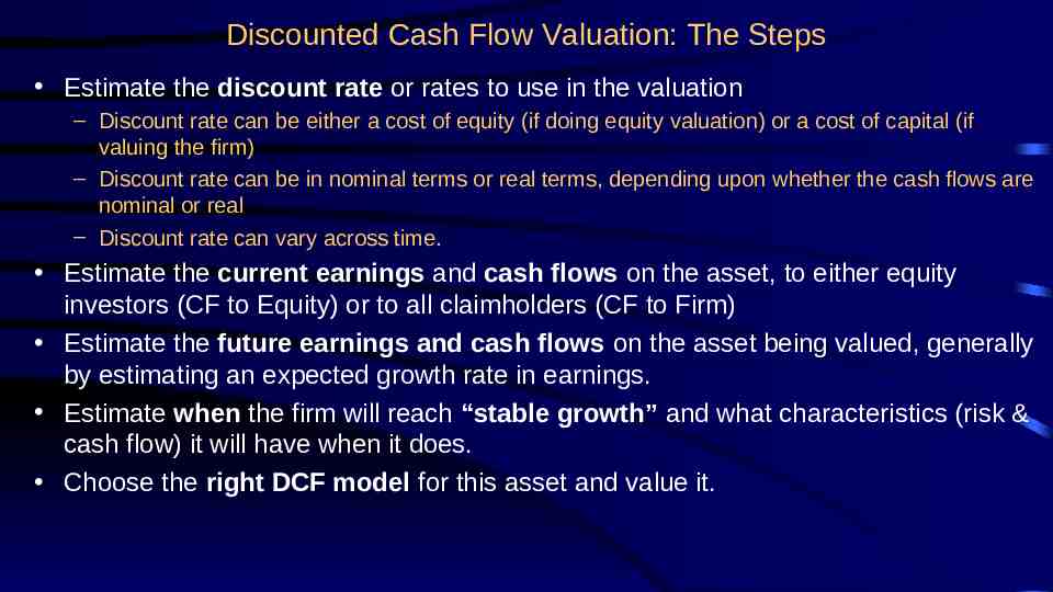
Discounted Cash Flow Valuation: The Steps Estimate the discount rate or rates to use in the valuation – Discount rate can be either a cost of equity (if doing equity valuation) or a cost of capital (if valuing the firm) – Discount rate can be in nominal terms or real terms, depending upon whether the cash flows are nominal or real – Discount rate can vary across time. Estimate the current earnings and cash flows on the asset, to either equity investors (CF to Equity) or to all claimholders (CF to Firm) Estimate the future earnings and cash flows on the asset being valued, generally by estimating an expected growth rate in earnings. Estimate when the firm will reach “stable growth” and what characteristics (risk & cash flow) it will have when it does. Choose the right DCF model for this asset and value it.
Discounted Cash Flow Valuation: The Inputs
The Key Inputs in DCF Valuation Discount Rate – Cost of Equity, in valuing equity – Cost of Capital, in valuing the firm Cash Flows – Cash Flows to Equity – Cash Flows to Firm Growth (to get future cash flows) – Growth in Equity Earnings – Growth in Firm Earnings (Operating Income)
I. Estimating Discount Rates DCF Valuation
Estimating Inputs: Discount Rates Critical ingredient in discounted cashflow valuation. Errors in estimating the discount rate or mismatching cashflows and discount rates can lead to serious errors in valuation. At an intuitive level, the discount rate used should be consistent with both the riskiness and the type of cashflow being discounted. – Equity versus Firm: If the cash flows being discounted are cash flows to equity, the appropriate discount rate is a cost of equity. If the cash flows are cash flows to the firm, the appropriate discount rate is the cost of capital. – Currency: The currency in which the cash flows are estimated should also be the currency in which the discount rate is estimated. – Nominal versus Real: If the cash flows being discounted are nominal cash flows (i.e., reflect expected inflation), the discount rate should be nominal
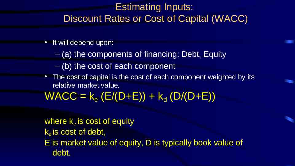
Estimating Inputs: Discount Rates or Cost of Capital (WACC) It will depend upon: – (a) the components of financing: Debt, Equity – (b) the cost of each component The cost of capital is the cost of each component weighted by its relative market value. WACC ke (E/(D E)) kd (D/(D E)) where ke is cost of equity kd is cost of debt, E is market value of equity, D is typically book value of debt.
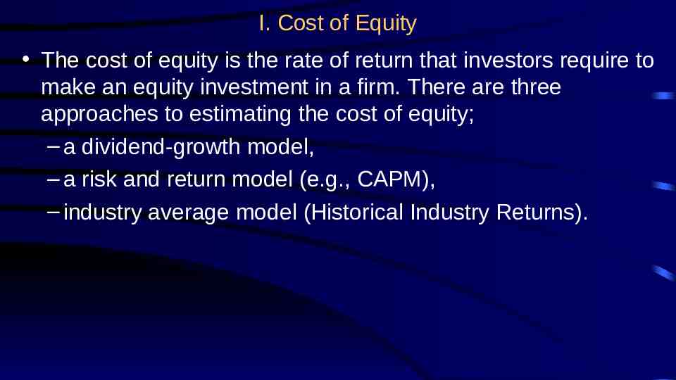
I. Cost of Equity The cost of equity is the rate of return that investors require to make an equity investment in a firm. There are three approaches to estimating the cost of equity; – a dividend-growth model, – a risk and return model (e.g., CAPM), – industry average model (Historical Industry Returns).
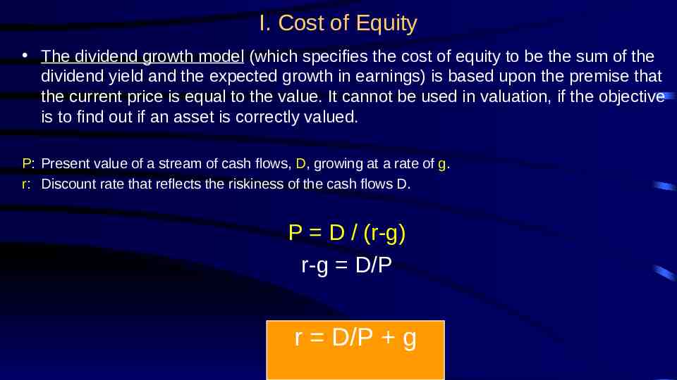
I. Cost of Equity The dividend growth model (which specifies the cost of equity to be the sum of the dividend yield and the expected growth in earnings) is based upon the premise that the current price is equal to the value. It cannot be used in valuation, if the objective is to find out if an asset is correctly valued. P: Present value of a stream of cash flows, D, growing at a rate of g. r: Discount rate that reflects the riskiness of the cash flows D. P D / (r-g) r-g D/P r D/P g
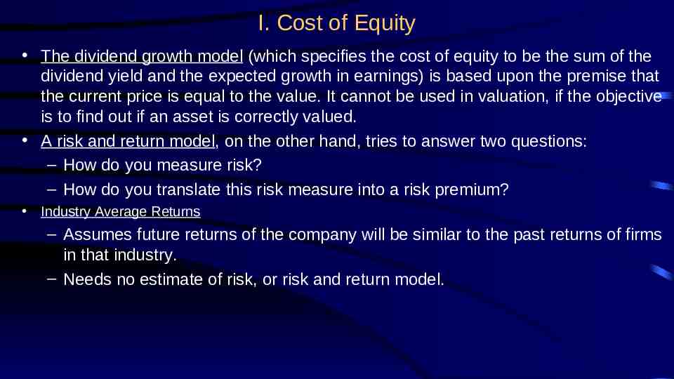
I. Cost of Equity The dividend growth model (which specifies the cost of equity to be the sum of the dividend yield and the expected growth in earnings) is based upon the premise that the current price is equal to the value. It cannot be used in valuation, if the objective is to find out if an asset is correctly valued. A risk and return model, on the other hand, tries to answer two questions: – How do you measure risk? – How do you translate this risk measure into a risk premium? Industry Average Returns – Assumes future returns of the company will be similar to the past returns of firms in that industry. – Needs no estimate of risk, or risk and return model.
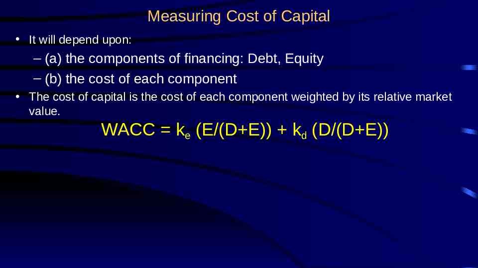
Measuring Cost of Capital It will depend upon: – (a) the components of financing: Debt, Equity – (b) the cost of each component The cost of capital is the cost of each component weighted by its relative market value. WACC ke (E/(D E)) kd (D/(D E))
The Cost of Debt The cost of debt is the market interest rate that the firm has to pay on its borrowing. It will depend upon three components- (a) The general level of interest rates (b) The default premium (c) The firm's tax rate
What the cost of debt is and is not. The cost of debt is – the rate at which the company can borrow at today – corrected for the tax benefit it gets for interest payments. Cost of debt kd Interest Rate on Debt (1 - Tax rate) The cost of debt is not – the interest rate at which the company obtained the debt it has on its books.
Estimating the Cost of Debt If the firm has bonds outstanding, and the bonds are traded, the yield to maturity on a long-term, straight (no special features) bond can be used as the interest rate. If the firm is rated, use the rating and a typical default spread on bonds with that rating to estimate the cost of debt. If the firm is not rated, – and it has recently borrowed long term from a bank, use the interest rate on the borrowing or – estimate a synthetic rating for the company, and use the synthetic rating to arrive at a default spread and a cost of debt The cost of debt has to be estimated in the same currency as the cost of equity and the cash flows in the valuation.
Calculate the weights of each component Use target/average debt weights rather than project-specific weights. Use market value weights for debt and equity. – The cost of capital is a measure of how much it would cost you to go out and raise the financing to acquire the business you are valuing today. Since you have to pay market prices for debt and equity, the cost of capital is better estimated using market value weights. – Book values are often misleading and outdated.
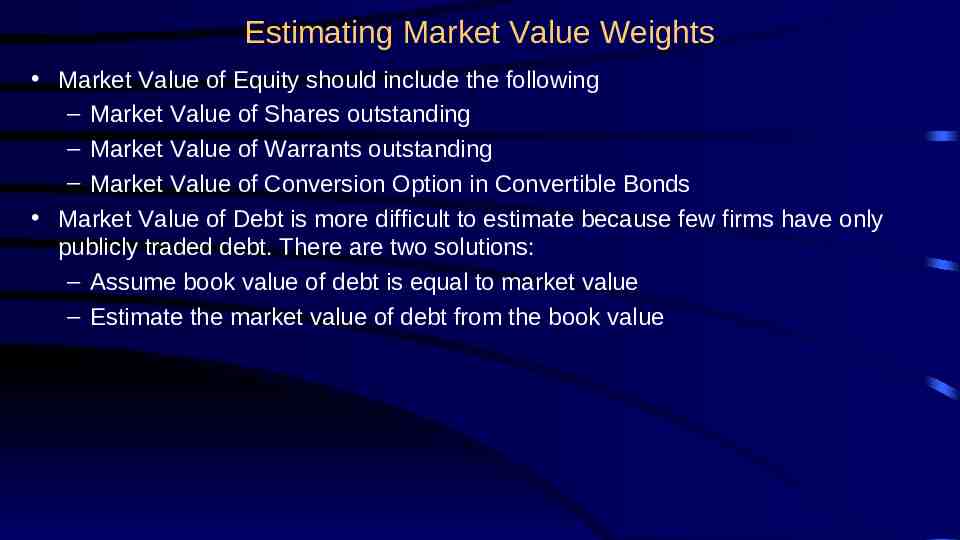
Estimating Market Value Weights Market Value of Equity should include the following – Market Value of Shares outstanding – Market Value of Warrants outstanding – Market Value of Conversion Option in Convertible Bonds Market Value of Debt is more difficult to estimate because few firms have only publicly traded debt. There are two solutions: – Assume book value of debt is equal to market value – Estimate the market value of debt from the book value
II. Estimating Cash Flows DCF Valuation
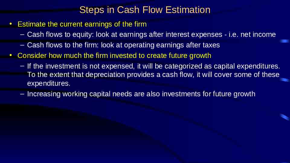
Steps in Cash Flow Estimation Estimate the current earnings of the firm – Cash flows to equity: look at earnings after interest expenses - i.e. net income – Cash flows to the firm: look at operating earnings after taxes Consider how much the firm invested to create future growth – If the investment is not expensed, it will be categorized as capital expenditures. To the extent that depreciation provides a cash flow, it will cover some of these expenditures. – Increasing working capital needs are also investments for future growth
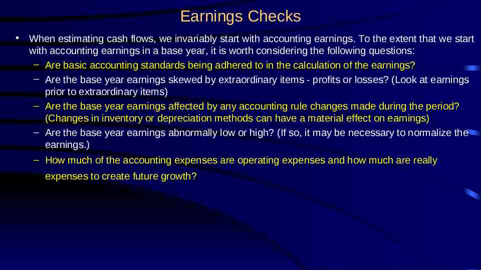
Earnings Checks When estimating cash flows, we invariably start with accounting earnings. To the extent that we start with accounting earnings in a base year, it is worth considering the following questions: – Are basic accounting standards being adhered to in the calculation of the earnings? – Are the base year earnings skewed by extraordinary items - profits or losses? (Look at earnings prior to extraordinary items) – Are the base year earnings affected by any accounting rule changes made during the period? (Changes in inventory or depreciation methods can have a material effect on earnings) – Are the base year earnings abnormally low or high? (If so, it may be necessary to normalize the earnings.) – How much of the accounting expenses are operating expenses and how much are really expenses to create future growth?
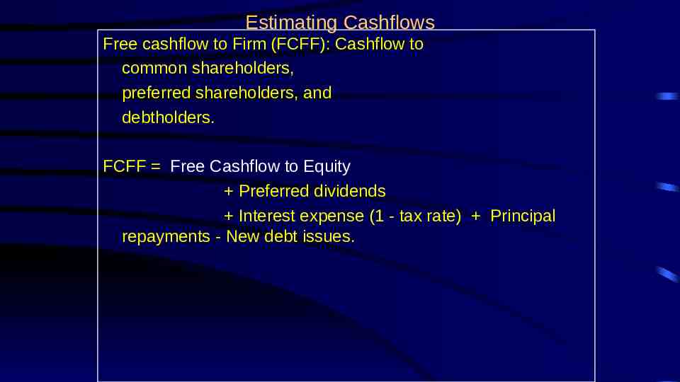
Estimating Cashflows Free cashflow to Firm (FCFF): Cashflow to common shareholders, preferred shareholders, and debtholders. FCFF Free Cashflow to Equity Preferred dividends Interest expense (1 - tax rate) Principal repayments - New debt issues.
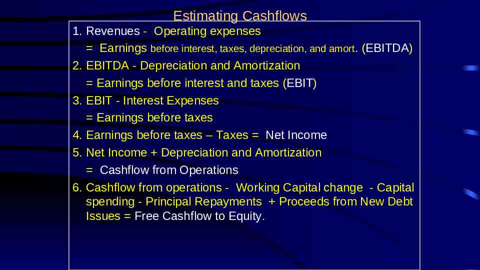
Estimating Cashflows 1. Revenues - Operating expenses Earnings before interest, taxes, depreciation, and amort. (EBITDA) 2. EBITDA - Depreciation and Amortization Earnings before interest and taxes (EBIT) 3. EBIT - Interest Expenses Earnings before taxes 4. Earnings before taxes – Taxes Net Income 5. Net Income Depreciation and Amortization Cashflow from Operations 6. Cashflow from operations - Working Capital change - Capital spending - Principal Repayments Proceeds from New Debt Issues Free Cashflow to Equity.
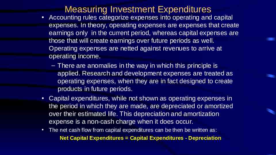
Measuring Investment Expenditures Accounting rules categorize expenses into operating and capital expenses. In theory, operating expenses are expenses that create earnings only in the current period, whereas capital expenses are those that will create earnings over future periods as well. Operating expenses are netted against revenues to arrive at operating income. – There are anomalies in the way in which this principle is applied. Research and development expenses are treated as operating expenses, when they are in fact designed to create products in future periods. Capital expenditures, while not shown as operating expenses in the period in which they are made, are depreciated or amortized over their estimated life. This depreciation and amortization expense is a non-cash charge when it does occur. The net cash flow from capital expenditures can be then be written as: Net Capital Expenditures Capital Expenditures - Depreciation
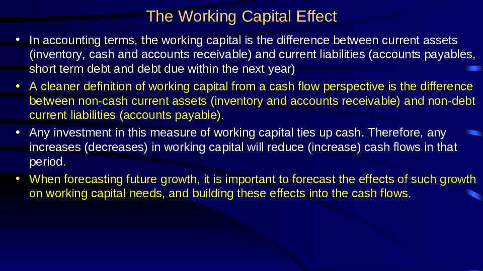
The Working Capital Effect In accounting terms, the working capital is the difference between current assets (inventory, cash and accounts receivable) and current liabilities (accounts payables, short term debt and debt due within the next year) A cleaner definition of working capital from a cash flow perspective is the difference between non-cash current assets (inventory and accounts receivable) and non-debt current liabilities (accounts payable). Any investment in this measure of working capital ties up cash. Therefore, any increases (decreases) in working capital will reduce (increase) cash flows in that period. When forecasting future growth, it is important to forecast the effects of such growth on working capital needs, and building these effects into the cash flows.
III. Estimating Growth DCF Valuation
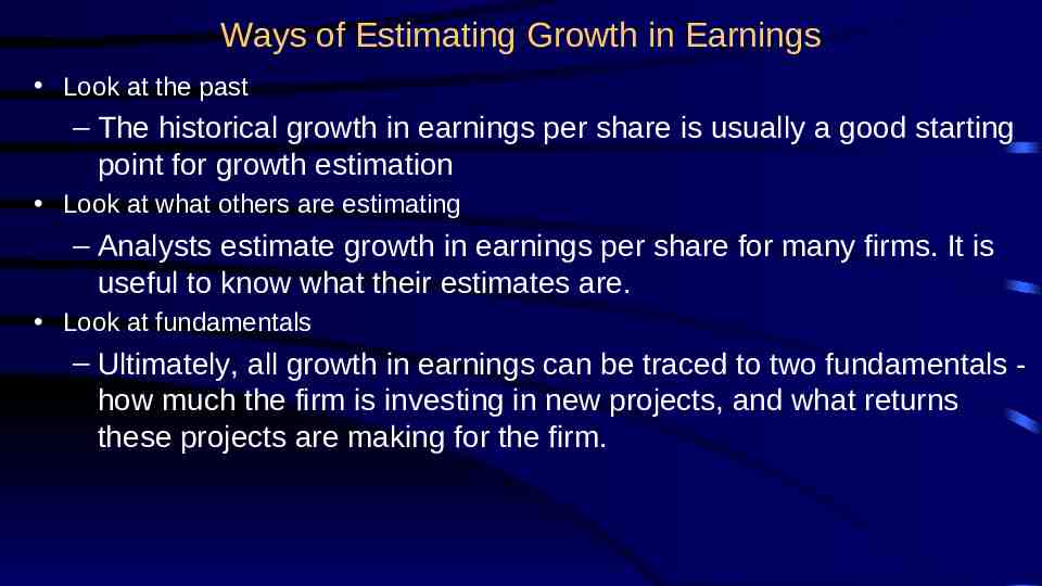
Ways of Estimating Growth in Earnings Look at the past – The historical growth in earnings per share is usually a good starting point for growth estimation Look at what others are estimating – Analysts estimate growth in earnings per share for many firms. It is useful to know what their estimates are. Look at fundamentals – Ultimately, all growth in earnings can be traced to two fundamentals how much the firm is investing in new projects, and what returns these projects are making for the firm.
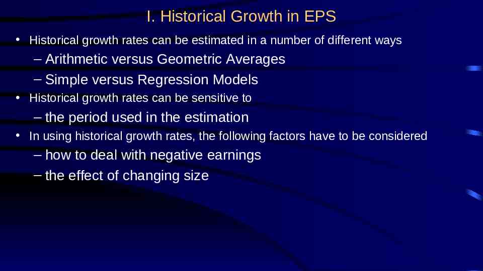
I. Historical Growth in EPS Historical growth rates can be estimated in a number of different ways – Arithmetic versus Geometric Averages – Simple versus Regression Models Historical growth rates can be sensitive to – the period used in the estimation In using historical growth rates, the following factors have to be considered – how to deal with negative earnings – the effect of changing size
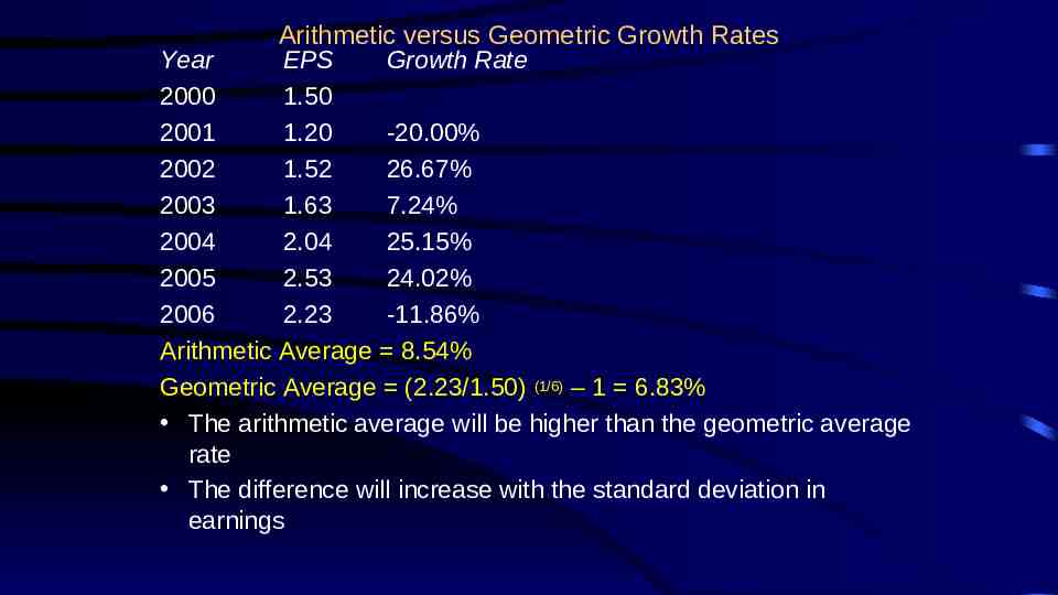
Arithmetic versus Geometric Growth Rates Year EPS Growth Rate 2000 1.50 2001 1.20 -20.00% 2002 1.52 26.67% 2003 1.63 7.24% 2004 2.04 25.15% 2005 2.53 24.02% 2006 2.23 -11.86% Arithmetic Average 8.54% Geometric Average (2.23/1.50) (1/6) – 1 6.83% The arithmetic average will be higher than the geometric average rate The difference will increase with the standard deviation in earnings
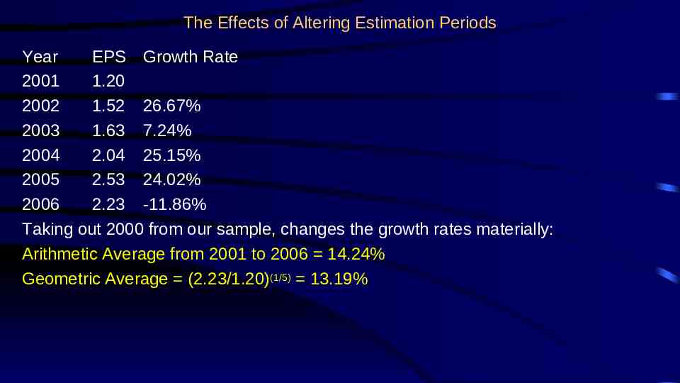
The Effects of Altering Estimation Periods Year EPS Growth Rate 2001 1.20 2002 1.52 26.67% 2003 1.63 7.24% 2004 2.04 25.15% 2005 2.53 24.02% 2006 2.23 -11.86% Taking out 2000 from our sample, changes the growth rates materially: Arithmetic Average from 2001 to 2006 14.24% Geometric Average (2.23/1.20)(1/5) 13.19%
Dealing with Negative Earnings When the earnings in the starting period are negative, the growth rate cannot be estimated. (0.30/-0.05 -600%) When earnings are negative, the growth rate is meaningless. Thus, while the growth rate can be estimated, it does not tell you much about the future.
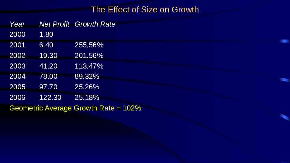
The Effect of Size on Growth Year Net Profit Growth Rate 2000 1.80 2001 6.40 255.56% 2002 19.30 201.56% 2003 41.20 113.47% 2004 78.00 89.32% 2005 97.70 25.26% 2006 122.30 25.18% Geometric Average Growth Rate 102%
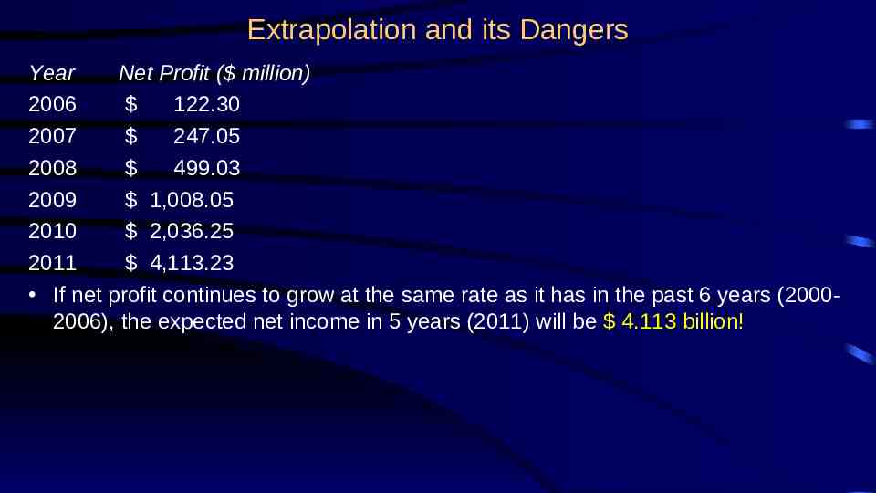
Extrapolation and its Dangers Year Net Profit ( million) 2006 122.30 2007 247.05 2008 499.03 2009 1,008.05 2010 2,036.25 2011 4,113.23 If net profit continues to grow at the same rate as it has in the past 6 years (20002006), the expected net income in 5 years (2011) will be 4.113 billion!
Propositions about Historical Growth Proposition 1: And in today already walks tomorrow. Coleridge Proposition 2: You cannot plan the future by the past Burke Proposition 3: Past growth carries the most information for firms whose size and business mix have not changed during the estimation period, and are not expected to change during the forecasting period. Proposition 4: Past growth carries the least information for firms in transition (from small to large, from one business to another.)
II. Analyst Forecasts of Growth While the job of an analyst is to find under and over valued stocks in the sectors that they follow, a significant proportion of an analyst’s time (outside of selling) is spent forecasting earnings per share. – Most of this time, in turn, is spent forecasting earnings per share in the next earnings report – While many analysts forecast expected growth in earnings per share over the next 5 years, the analysis and information (generally) that goes into this estimate is far more limited. Analyst forecasts of earnings per share and expected growth are widely disseminated by services such as Zacks and IBES, at least for U.S companies.
How good are analysts at forecasting growth? Analysts forecasts of EPS tend to be closer to the actual EPS than simple time series models, but the differences tend to be small The advantage that analysts have over time series models – tends to decrease with the forecast period (next quarter versus 5 years) – tends to be greater for larger firms than for smaller firms – tends to be greater at the industry level than at the company level Forecasts of growth (and revisions thereof) tend to be highly correlated across analysts.
Are some analysts more equal than others? A study of All-America Analysts (chosen by Institutional Investor) found that – There is no evidence that analysts who are chosen for the All-America Analyst team were chosen because they were better forecasters of earnings. (Their median forecast error in the quarter prior to being chosen was 30%; the median forecast error of other analysts was 28%) – However, in the calendar year following being chosen as All-America analysts, these analysts become slightly better forecasters than their less fortunate brethren. (The median forecast error for All-America analysts is 2% lower than the median forecast error for other analysts.) – Earnings revisions made by All-America analysts tend to have a much greater impact on the stock price than revisions from other analysts – The recommendations made by the All America analysts have a greater impact on stock prices (3% on buys; 4.7% on sells). For these recommendations the price changes are sustained, and they continue to rise in the following period (2.4% for buys; 13.8% for the sells).
The Five Deadly Sins of an Analyst Tunnel Vision: Becoming so focused on the sector and valuations within the sector that they lose sight of the bigger picture. Lemmingitis:Strong urge felt by analysts to change recommendations and revise earnings estimates when other analysts do the same. Stockholm Syndrome: Refers to analysts who start identifying with the managers of the firms that they are supposed to follow. Factophobia (generally is coupled with delusions of being a famous story teller): Tendency to base a recommendation on a “story” coupled with a refusal to face the facts. Dr. Jekyll/Mr.Hyde: Analyst who thinks her primary job is to bring in investment banking business to the firm.
Propositions about Analyst Growth Rates Proposition 1: There is far less private information and far more public information in most analyst forecasts than is generally claimed. Proposition 2: The biggest source of private information for analysts remains the company itself which might explain – why there are more buy recommendations than sell recommendations (information bias and the need to preserve sources) – why there is such a high correlation across analysts forecasts and revisions – why All-America analysts become better forecasters than other analysts after they are chosen to be part of the team. Proposition 3: There is value to knowing what analysts are forecasting as earnings growth for a firm. There is, however, danger when they agree too much (lemmingitis) and when they agree too little (in which case the information that they have is so noisy as to be useless).
IV. Growth Patterns Discounted Cashflow Valuation
Stable Growth and Terminal Value When a firm’s cash flows grow at a “constant” rate forever, the present value of those cash flows can be written as: Value Expected Cash Flow Next Period / (r - g) where, r Discount rate (Cost of Equity or Cost of Capital) g Expected growth rate This “constant” growth rate is called a stable growth rate and cannot be higher than the growth rate of the economy in which the firm operates. While companies can maintain high growth rates for extended periods, they will all approach “stable growth” at some point in time. When they do approach stable growth, the valuation formula above can be used to estimate the “terminal value” of all cash flows beyond.
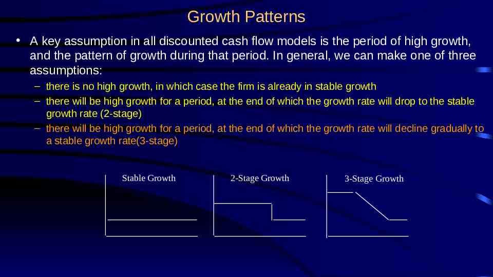
Growth Patterns A key assumption in all discounted cash flow models is the period of high growth, and the pattern of growth during that period. In general, we can make one of three assumptions: – there is no high growth, in which case the firm is already in stable growth – there will be high growth for a period, at the end of which the growth rate will drop to the stable growth rate (2-stage) – there will be high growth for a period, at the end of which the growth rate will decline gradually to a stable growth rate(3-stage) Stable Growth 2-Stage Growth 3-Stage Growth
Determinants of Growth Patterns Size of the firm – Success usually makes a firm larger. As firms become larger, it becomes much more difficult for them to maintain high growth rates Current growth rate – While past growth is not always a reliable indicator of future growth, there is a correlation between current growth and future growth. Thus, a firm growing at 30% currently probably has higher growth and a longer expected growth period than one growing 10% a year now. Barriers to entry and differential advantages – Ultimately, high growth comes from high project returns, which, in turn, comes from barriers to entry and differential advantages. – The question of how long growth will last and how high it will be can therefore be framed as a question about what the barriers to entry are, how long they will stay up and how strong they will remain.
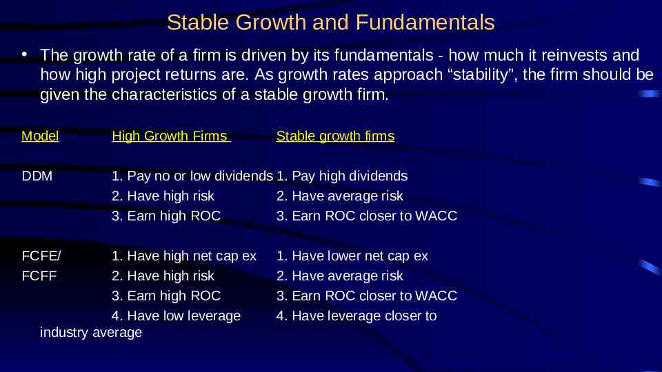
Stable Growth and Fundamentals The growth rate of a firm is driven by its fundamentals - how much it reinvests and how high project returns are. As growth rates approach “stability”, the firm should be given the characteristics of a stable growth firm. Model High Growth Firms DDM 1. Pay no or low dividends 1. Pay high dividends 2. Have high risk 2. Have average risk 3. Earn high ROC 3. Earn ROC closer to WACC FCFE/ FCFF 1. Have high net cap ex 2. Have high risk 3. Earn high ROC 4. Have low leverage industry average Stable growth firms 1. Have lower net cap ex 2. Have average risk 3. Earn ROC closer to WACC 4. Have leverage closer to
V. Beyond Inputs: Choosing and Using the Right Model Discounted Cashflow Valuation
Summarizing the Inputs In summary, at this stage in the process, we should have an estimate of the – the current cash flows on the investment, either to equity investors (dividends or free cash flows to equity) or to the firm (cash flow to the firm) – the current cost of equity and/or capital on the investment – the expected growth rate in earnings, based upon historical growth, analysts forecasts and/or fundamentals. The next step in the process is deciding – which cash flow to discount, which should indicate – which discount rate needs to be estimated and – what pattern we will assume growth to follow.
Which cash flow should I discount? Use Equity Valuation (a) for firms which have stable leverage, whether high or not, and (b) if equity (stock) is being valued Use Firm Valuation (a) for firms which have leverage which is too high or too low, and expect to change the leverage over time, because debt payments and issues do not have to be factored in the cash flows and the discount rate (cost of capital) does not change dramatically over time. (b) for firms for which you have partial information on leverage (eg: interest expenses are missing.) (c) in all other cases, where you are more interested in valuing the firm than the equity. (Value Consulting?)
Given cash flows to equity, should I discount dividends or FCFE? Use the Dividend Discount Model – (a) For firms which pay dividends (and repurchase stock) which are close to the Free Cash Flow to Equity (over a extended period) – (b)For firms where FCFE are difficult to estimate (Example: Banks and Financial Service companies) Use the FCFE Model – (a) For firms which pay dividends which are significantly higher or lower than the Free Cash Flow to Equity. (What is significant? . As a rule of thumb, if dividends are less than 80% of FCFE or dividends are greater than 110% of FCFE over a 5-year period, use the FCFE model) – (b) For firms where dividends are not available (Example: Private Companies, IPOs)
What discount rate should I use? Cost of Equity versus Cost of Capital – If discounting cash flows to equity - Cost of Equity – If discounting cash flows to the firm- Cost of Capital What currency should the discount rate (risk free rate) be in? – Match the currency in which you estimate the risk free rate to the currency of your cash flows Should I use real or nominal cash flows? – If discounting real cash flows- real cost of capital – If nominal cash flows - nominal cost of capital – If inflation is low ( 10%), stick with nominal cash flows since taxes are based upon nominal income – If inflation is high ( 10%) switch to real cash flows
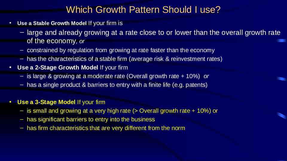
Which Growth Pattern Should I use? Use a Stable Growth Model If your firm is – large and already growing at a rate close to or lower than the overall growth rate of the economy, or – constrained by regulation from growing at rate faster than the economy – has the characteristics of a stable firm (average risk & reinvestment rates) Use a 2-Stage Growth Model If your firm – is large & growing at a moderate rate (Overall growth rate 10%) or – has a single product & barriers to entry with a finite life (e.g. patents) Use a 3-Stage Model If your firm – is small and growing at a very high rate ( Overall growth rate 10%) or – has significant barriers to entry into the business – has firm characteristics that are very different from the norm
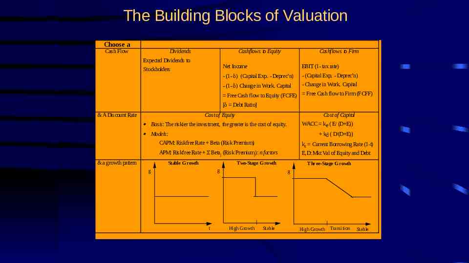
The Building Blocks of Valuation Choose a Cash Flow Dividends Cashflows to Equity Expected Dividends to Stockholders Cashflows to Firm Net Income EBIT (1- tax rate) - (1- ) (Capital Exp. - Deprec’n) - (Capital Exp. - Deprec’n) - (1- ) Change in Work. Capital - Change in Work. Capital Free Cash flow to Equity (FCFE) Free Cash flow to Firm (FCFF) [ Debt Ratio] & A Discount Rate Cost of Equity Cost of Capital WACC ke ( E/ (D E)) Basis: The riskier the investment, the greater is the cost of equity. Models: CAPM: Riskfree Rate Beta (Risk Premium) kd ( D/(D E)) kd Current Borrowing Rate (1-t) APM: Riskfree Rate Betaj (Risk Premiumj): n factors & a growth pattern Stable G rowth E,D: Mkt Val of Equity and Debt Two-Stage Growth g g g t Three-Stage Growth High Growth Stable High Growth Transition Stable