WK3 – Multi Layer Perceptron Contents MLP Model BP Algorithm


59 Slides934.00 KB
WK3 – Multi Layer Perceptron Contents MLP Model BP Algorithm Approxim. CS 476: Networks of Neural Computation WK3 – Multi Layer Perceptron Model Selec. BP & Opt. Conclusions Dr. Stathis Kasderidis Dept. of Computer Science University of Crete Spring Semester, 2009 CS 476: Networks of Neural Computation, CSD, UOC, 2009
Contents Contents MLP Model BP Algorithm MLP model details Back-propagation algorithm XOR Example Approxim. Heuristics for Back-propagation Model Selec. Heuristics for learning rate BP & Opt. Approximation of functions Conclusions Generalisation Model selection through cross-validation Conguate-Gradient method for BP CS 476: Networks of Neural Computation, CSD, UOC, 2009
Contents II Contents MLP Model BP Algorithm Advantages and disadvantages of BP Types of problems for applying BP Conclusions Approxim. Model Selec. BP & Opt. Conclusions CS 476: Networks of Neural Computation, CSD, UOC, 2009
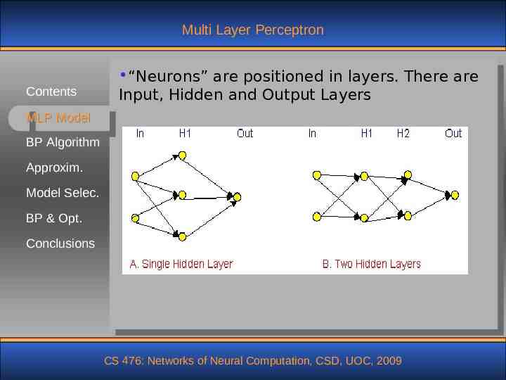
Multi Layer Perceptron Contents “Neurons” are positioned in layers. There are Input, Hidden and Output Layers MLP Model BP Algorithm Approxim. Model Selec. BP & Opt. Conclusions CS 476: Networks of Neural Computation, CSD, UOC, 2009
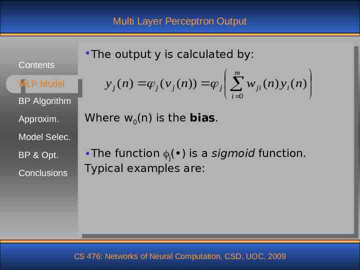
Multi Layer Perceptron Output Contents MLP Model BP Algorithm Approxim. The output y is calculated by: m y j ( n) j (v j ( n)) j w ji ( n) yi ( n) i 0 Where w0(n) is the bias. Model Selec. BP & Opt. Conclusions The function j( ) is a sigmoid function. Typical examples are: CS 476: Networks of Neural Computation, CSD, UOC, 2009
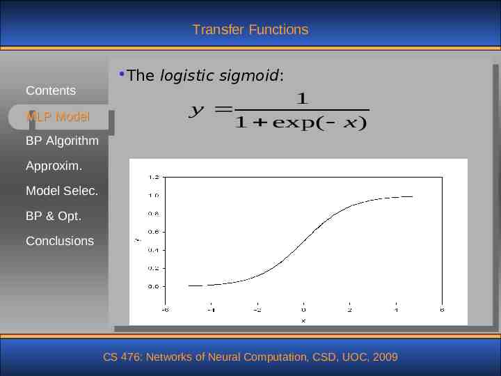
Transfer Functions Contents MLP Model The logistic sigmoid: 1 y 1 exp( x ) BP Algorithm Approxim. Model Selec. BP & Opt. Conclusions CS 476: Networks of Neural Computation, CSD, UOC, 2009
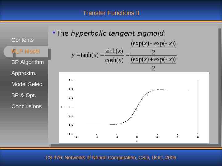
Transfer Functions II Contents MLP Model BP Algorithm Approxim. The hyperbolic tangent sigmoid: (exp( x) exp( x)) sinh( x) 2 y tanh( x) cosh( x) (exp( x) exp( x)) 2 Model Selec. BP & Opt. Conclusions CS 476: Networks of Neural Computation, CSD, UOC, 2009
Learning Algorithm Assume that a set of examples {x(n),d(n)}, Contents n 1, ,N is given. x(n) is the input vector of dimension m0 and d(n) is the desired response MLP Model vector of dimension M BP Algorithm Thus an error signal, ej(n) dj(n)-yj(n) can be Approxim. defined for the output neuron j. Model Selec. We can derive a learning algorithm for an MLP BP & Opt. by assuming an optimisation approach which is based on the steepest descent direction, I.e. Conclusions w(n) - g(n) Where g(n) is the gradient vector of the cost function and is the learning rate. CS 476: Networks of Neural Computation, CSD, UOC, 2009
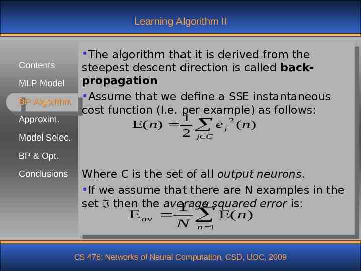
Learning Algorithm II The algorithm that it is derived from the Contents steepest descent direction is called backpropagation MLP Model BP Algorithm Assume that we define a SSE instantaneous cost function (I.e. per example) as follows: 1 Approxim. 2 ( n) e j ( n) 2 j C Model Selec. BP & Opt. Conclusions Where C is the set of all output neurons. If we assume that there are N examples in the set then the average 1 N squared error is: av N ( n) n 1 CS 476: Networks of Neural Computation, CSD, UOC, 2009
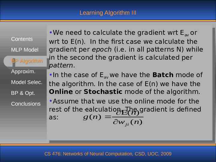
Learning Algorithm III We need to calculate the gradient wrt Eav or Contents wrt to E(n). In the first case we calculate the MLP Model gradient per epoch (i.e. in all patterns N) while in the second the gradient is calculated per BP Algorithm pattern. Approxim. In the case of Eav we have the Batch mode of Model Selec. the algorithm. In the case of E(n) we have the Online or Stochastic mode of the algorithm. BP & Opt. Assume that we use the online mode for the Conclusions rest of the calculation. The ( n)gradient is defined g ( n) as: w ji ( n) CS 476: Networks of Neural Computation, CSD, UOC, 2009
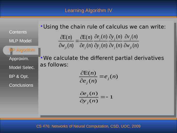
Learning Algorithm IV Contents MLP Model BP Algorithm Approxim. Model Selec. BP & Opt. Conclusions Using the chain rule of calculus we can write: (n) (n) e j (n) y j (n) v j (n) w ji (n) e j (n) y j (n) v j (n) w ji (n) We calculate the different partial derivatives as follows: ( n) e j ( n) e j ( n) e j ( n) y j ( n) 1 CS 476: Networks of Neural Computation, CSD, UOC, 2009
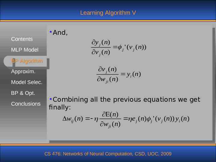
Learning Algorithm V Contents MLP Model And, y j (n) v j (n) j ' (v j (n)) BP Algorithm Approxim. v j ( n) Model Selec. w ji ( n) BP & Opt. Conclusions yi ( n ) Combining all the previous equations we get finally: ( n) wij (n) e j (n) j ' (v j (n)) yi (n) w ji (n) CS 476: Networks of Neural Computation, CSD, UOC, 2009
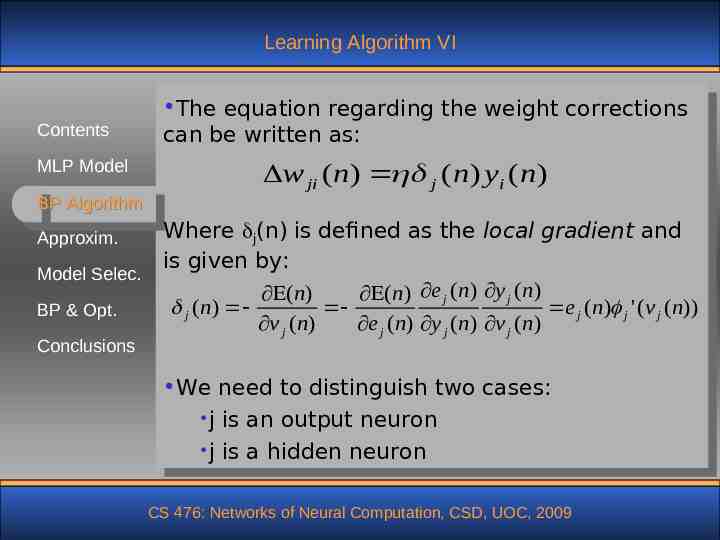
Learning Algorithm VI Contents MLP Model BP Algorithm Approxim. Model Selec. BP & Opt. Conclusions The equation regarding the weight corrections can be written as: w ji ( n) j (n) yi (n) Where j(n) is defined as the local gradient and is given by: ( n) (n) e j ( n) y j ( n) j ( n) e j (n) j ' (v j (n)) v j (n) e j (n) y j (n) v j (n) We need to distinguish two cases: j is an output neuron j is a hidden neuron CS 476: Networks of Neural Computation, CSD, UOC, 2009
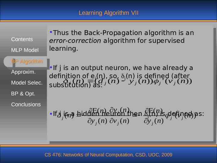
Learning Algorithm VII Contents MLP Model BP Algorithm Approxim. Model Selec. Thus the Back-Propagation algorithm is an error-correction algorithm for supervised learning. If j is an output neuron, we have already a definition of ej(n), so, j(n) is defined (after j ( n) ( d j (n) y j ( n)) j ' (v j ( n)) substitution) as: BP & Opt. Conclusions y j (n) ( n ) ( n)is defined as: a hidden neuron then (n) If j jis (n) j j ' (v j (n)) y j (n) v j (n) y j (n) CS 476: Networks of Neural Computation, CSD, UOC, 2009
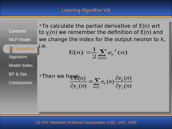
Learning Algorithm VIII To calculate the partial derivative of E(n) wrt Contents to yj(n) we remember the definition of E(n) and MLP Model we change the index for the output neuron to k, i.e. BP Algorithm 1 2 ( n) ek ( n) 2 k C Approxim. Model Selec. BP & Opt. Conclusions Then we have: e (n) (n) ek ( n) k y j (n) k C y j (n) CS 476: Networks of Neural Computation, CSD, UOC, 2009
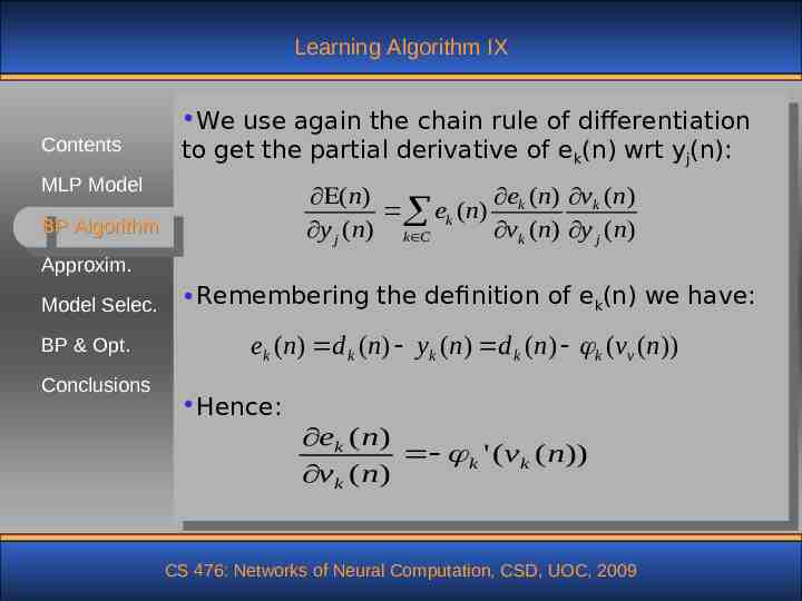
Learning Algorithm IX Contents We use again the chain rule of differentiation to get the partial derivative of ek(n) wrt yj(n): MLP Model ek (n) vk (n) (n) ek ( n) y j ( n) k C vk (n) y j ( n) BP Algorithm Approxim. Model Selec. BP & Opt. Conclusions Remembering the definition of ek(n) we have: ek (n) d k (n) yk (n) d k (n) k (vv (n)) Hence: ek ( n) k ' (vk ( n)) vk ( n) CS 476: Networks of Neural Computation, CSD, UOC, 2009
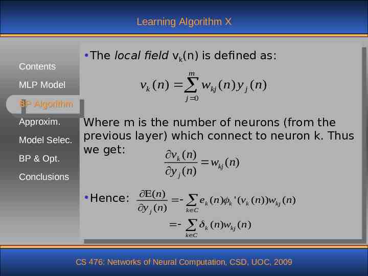
Learning Algorithm X Contents MLP Model The local field vk(n) is defined as: m vk (n) wkj (n) y j ( n) j 0 BP Algorithm Approxim. Model Selec. BP & Opt. Conclusions Where m is the number of neurons (from the previous layer) which connect to neuron k. Thus we get: vk (n) wkj ( n) y j ( n) Hence: (n) ek (n) k ' (vk (n))wkj (n) y j (n) k C k ( n)wkj ( n) k C CS 476: Networks of Neural Computation, CSD, UOC, 2009
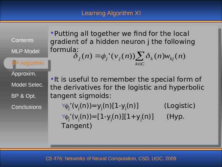
Learning Algorithm XI Contents MLP Model Putting all together we find for the local gradient of a hidden neuron j the following formula: j (n) j ' (v j (n)) k (n)wkj (n) BP Algorithm Approxim. Model Selec. BP & Opt. Conclusions k C It is useful to remember the special form of the derivatives for the logistic and hyperbolic tangent sigmoids: ’(v (n)) y (n)[1-y (n)] (Logistic) j j j j ’(v (n)) [1-y (n)][1 y (n)] j j j j (Hyp. Tangent) CS 476: Networks of Neural Computation, CSD, UOC, 2009
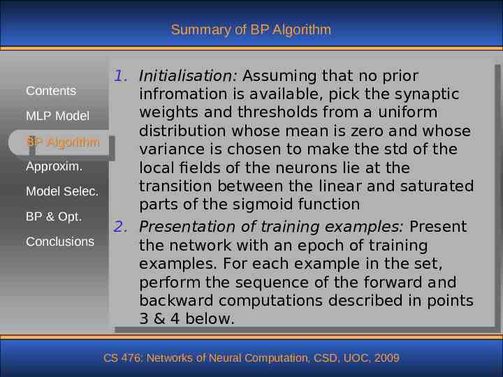
Summary of BP Algorithm 1. Initialisation: Assuming that no prior Contents infromation is available, pick the synaptic weights and thresholds from a uniform MLP Model distribution whose mean is zero and whose BP Algorithm variance is chosen to make the std of the Approxim. local fields of the neurons lie at the transition between the linear and saturated Model Selec. parts of the sigmoid function BP & Opt. 2. Presentation of training examples: Present Conclusions the network with an epoch of training examples. For each example in the set, perform the sequence of the forward and backward computations described in points 3 & 4 below. CS 476: Networks of Neural Computation, CSD, UOC, 2009
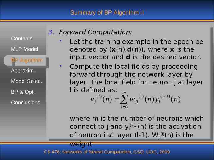
Summary of BP Algorithm II 3. Forward Computation: Contents Let the training example in the epoch be MLP Model denoted by (x(n),d(n)), where x is the input vector and d is the desired vector. BP Algorithm Compute the local fields by proceeding Approxim. forward through the network layer by Model Selec. layer. The local field for neuron j at layer l is defined as: m BP & Opt. (l ) Conclusions (l ) v j ( n) w ji (n) yi ( l 1) ( n) i 0 where m is the number of neurons which connect to j and yi(l-1)(n) is the activation of neuron i at layer (l-1). Wji(l)(n) is the weight CS 476: Networks of Neural Computation, CSD, UOC, 2009
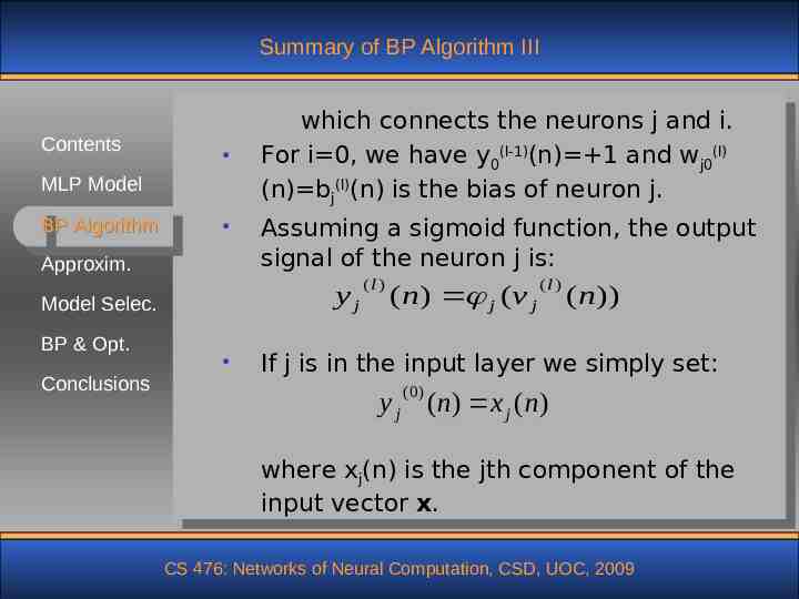
Summary of BP Algorithm III Contents MLP Model BP Algorithm Approxim. Conclusions Assuming a sigmoid function, the output signal of the neuron j is: yj Model Selec. BP & Opt. which connects the neurons j and i. For i 0, we have y0(l-1)(n) 1 and wj0(l) (n) bj(l)(n) is the bias of neuron j. (l ) ( n) j (v j (l ) ( n)) If j is in the input layer we simply set: (0) y j ( n) x j ( n) where xj(n) is the jth component of the input vector x. CS 476: Networks of Neural Computation, CSD, UOC, 2009
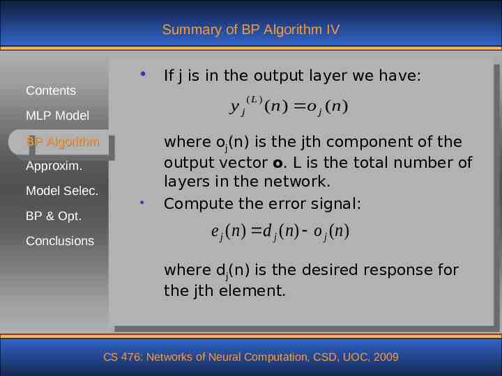
Summary of BP Algorithm IV Contents yj MLP Model BP Algorithm Approxim. Model Selec. BP & Opt. Conclusions If j is in the output layer we have: ( L) ( n) o j ( n) where oj(n) is the jth component of the output vector o. L is the total number of layers in the network. Compute the error signal: e j (n) d j (n) o j (n) where dj(n) is the desired response for the jth element. CS 476: Networks of Neural Computation, CSD, UOC, 2009
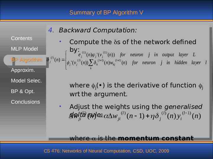
Summary of BP Algorithm V 4. Backward Computation: Contents MLP Model BP Algorithm j Approxim. (l ) e j (n) j ' (v j (n)) for neuron j in output layer L (l ) ( l 1) ( l 1) (n) j ' (v j (n)) k (n) wkj (n) for neuron j in hidden layer l k Model Selec. where j( ) is the derivative of function j wrt the argument. BP & Opt. Conclusions Compute the s of the network defined by: ( L ) ( L) Adjust the weights using the generalised (l ) (l ) (l ) ( l 1) delta w ji (rule: n) w ji (n 1) j (n) yi (n) where is the momentum constant CS 476: Networks of Neural Computation, CSD, UOC, 2009
Summary of BP Algorithm VI Contents MLP Model BP Algorithm Approxim. Model Selec. BP & Opt. Conclusions 5. Iteration: Iterate the forward and backward computations of steps 3 & 4 by presenting new epochs of training examples until the stopping criterion is met. The order of presentation of examples should be randomised from epoch to epoch The momentum and the learning rate parameters typically change (usually decreased) as the number of training iterations increases. CS 476: Networks of Neural Computation, CSD, UOC, 2009
Stopping Criteria The BP algorithm is considered to have converged when the Euclidean norm of the gradient vector reaches a sufficiently small gradient threshold. The BP is considered to have converged when the absolute value of the change in the average square error per epoch is sufficiently small Contents MLP Model BP Algorithm Approxim. Model Selec. BP & Opt. Conclusions CS 476: Networks of Neural Computation, CSD, UOC, 2009
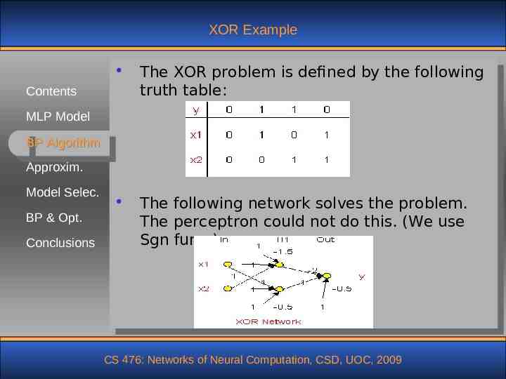
XOR Example The XOR problem is defined by the following truth table: The following network solves the problem. The perceptron could not do this. (We use Sgn func.) Contents MLP Model BP Algorithm Approxim. Model Selec. BP & Opt. Conclusions CS 476: Networks of Neural Computation, CSD, UOC, 2009
Heuristics for Back-Propagation Contents MLP Model BP Algorithm To speed the convergence of the backpropagation algorithm the following heuristics are applied: H1: Use sequential (online) vs batch update H2: Maximise information content Approxim. Model Selec. BP & Opt. Conclusions Use examples that produce largest error Use example which very different from all the previous ones H3: Use an antisymmetric activation function, such as the hyperbolic tangent. Antisymmetric means: (-x) - (x) CS 476: Networks of Neural Computation, CSD, UOC, 2009
Heuristics for Back-Propagation II H4: Use different target values inside a smaller range, different from the asymptotic values of the sigmoid H5: Normalise the inputs: Contents MLP Model BP Algorithm Approxim. Create zero-mean variables Model Selec. Decorrelate the variables BP & Opt. Scale the variables to have covariances approximately equal Conclusions H6: Initialise properly the weights. Use a zero mean distribution with variance of: w 1 m CS 476: Networks of Neural Computation, CSD, UOC, 2009
Heuristics for Back-Propagation III where m is the number of connections arriving to a neuron Contents MLP Model H7: Learn from hints BP Algorithm H8: Adapt the learning rates appropriately (see next section) Approxim. Model Selec. BP & Opt. Conclusions CS 476: Networks of Neural Computation, CSD, UOC, 2009
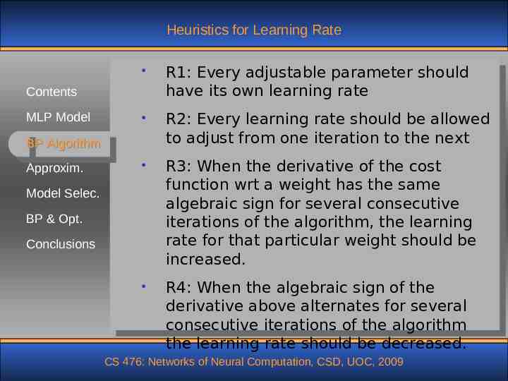
Heuristics for Learning Rate R1: Every adjustable parameter should have its own learning rate R2: Every learning rate should be allowed to adjust from one iteration to the next R3: When the derivative of the cost function wrt a weight has the same algebraic sign for several consecutive iterations of the algorithm, the learning rate for that particular weight should be increased. R4: When the algebraic sign of the derivative above alternates for several consecutive iterations of the algorithm the learning rate should be decreased. Contents MLP Model BP Algorithm Approxim. Model Selec. BP & Opt. Conclusions CS 476: Networks of Neural Computation, CSD, UOC, 2009
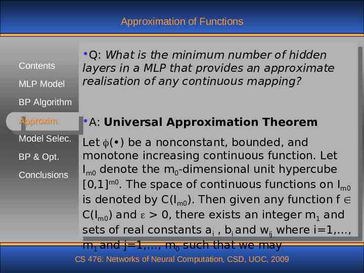
Approximation of Functions Contents MLP Model Q: What is the minimum number of hidden layers in a MLP that provides an approximate realisation of any continuous mapping? BP Algorithm Approxim. A: Universal Approximation Theorem Model Selec. Let ( ) be a nonconstant, bounded, and monotone increasing continuous function. Let Im0 denote the m0-dimensional unit hypercube [0,1]m0. The space of continuous functions on Im0 is denoted by C(Im0). Then given any function f C(Im0) and 0, there exists an integer m1 and sets of real constants ai , bi and wij where i 1, , m1 and j 1, , m0 such that we may BP & Opt. Conclusions CS 476: Networks of Neural Computation, CSD, UOC, 2009
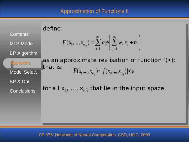
Approximation of Functions II Contents MLP Model BP Algorithm Approxim. Model Selec. define: m0 F ( x1 ,., xm0 ) ai wij x j bi i 1 j 1 m1 as an approximate realisation of function f( ); that is: F ( x1 ,., xm0 ) f ( x1 ,., xm0 ) BP & Opt. Conclusions for all x1, , xm0 that lie in the input space. CS 476: Networks of Neural Computation, CSD, UOC, 2009
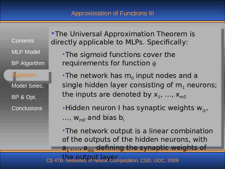
Approximation of Functions III Contents MLP Model The Universal Approximation Theorem is directly applicable to MLPs. Specifically: The BP Algorithm sigmoid functions cover the requirements for function Approxim. The BP & Opt. network has m0 input nodes and a single hidden layer consisting of m1 neurons; the inputs are denoted by x1, , xm0 Conclusions Hidden Model Selec. , wm0 The neuron I has synaptic weights wi1, and bias bi network output is a linear combination of the outputs of the hidden neurons, with a1 , , am1 defining the synaptic weights of the output layer CS 476: Networks of Neural Computation, CSD, UOC, 2009
Approximation of Functions IV Contents MLP Model BP Algorithm Approxim. Model Selec. BP & Opt. Conclusions The theorem is an existence theorem: It does not tell us exactly what is the number m1; it just says that exists!!! The theorem states that a single hidden layer is sufficient for an MLP to compute a uniform approximation to a given training set represented by the set of inputs x1, , xm0 and a desired output f(x1, , xm0). The theorem does not say however that a single hidden layer is optimum in the sense of the learning time, ease of implementation or generalisation. CS 476: Networks of Neural Computation, CSD, UOC, 2009
Approximation of Functions V Contents MLP Model BP Algorithm Approxim. Model Selec. BP & Opt. Conclusions Empirical knowledge shows that the number of data pairs that are needed in order to achieve a given error level is: W N O Where W is the total number of adjustable parameters of the model. There is mathematical support for this observation (but we will not analyse this further!) There is the “curse of dimensionality” for approximating functions in high-dimensional spaces. It is theoretically justified to use two hidden CS 476: Networks of Neural Computation, CSD, UOC, 2009 layers.
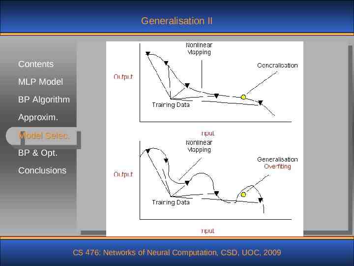
Generalisation Def: A network generalises well when the inputContents output mapping computed by the network is correct (or nearly so) for test data never used in MLP Model creating or training the network. It is assumed BP Algorithm that the test data are drawn form the population Approxim. used to generate the training data. Model Selec. BP & Opt. Conclusions We should try to approximate the true mechanism that generates the data; not the specific structure of the data in order to achieve the generalisation. If we learn the specific structure of the data we have overfitting or overtraining. CS 476: Networks of Neural Computation, CSD, UOC, 2009
Generalisation II Contents MLP Model BP Algorithm Approxim. Model Selec. BP & Opt. Conclusions CS 476: Networks of Neural Computation, CSD, UOC, 2009
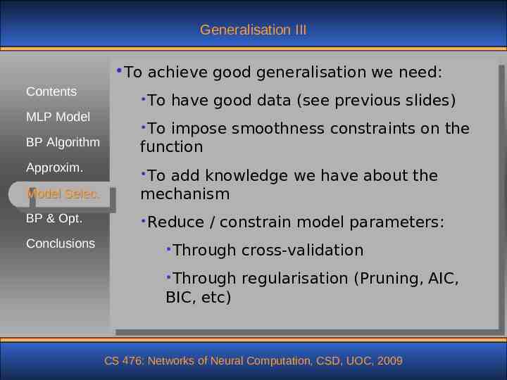
Generalisation III To achieve good generalisation we need: Contents MLP Model BP Algorithm Approxim. Model Selec. BP & Opt. Conclusions To have good data (see previous slides) To impose smoothness constraints on the function To add knowledge we have about the mechanism Reduce / constrain model parameters: Through cross-validation Through regularisation (Pruning, AIC, BIC, etc) CS 476: Networks of Neural Computation, CSD, UOC, 2009
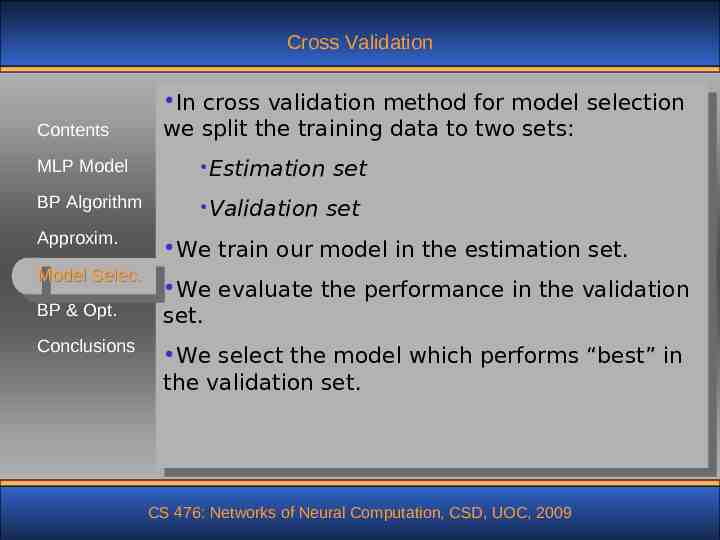
Cross Validation Contents In cross validation method for model selection we split the training data to two sets: MLP Model Estimation BP Algorithm Validation Approxim. Model Selec. BP & Opt. Conclusions set set We train our model in the estimation set. We evaluate the performance in the validation set. We select the model which performs “best” in the validation set. CS 476: Networks of Neural Computation, CSD, UOC, 2009
Cross Validation II Contents MLP Model There are variations of the method depending on the partition of the validation set. Typical variants are: BP Algorithm Method Approxim. Leave of early stopping k-out Model Selec. BP & Opt. Conclusions CS 476: Networks of Neural Computation, CSD, UOC, 2009
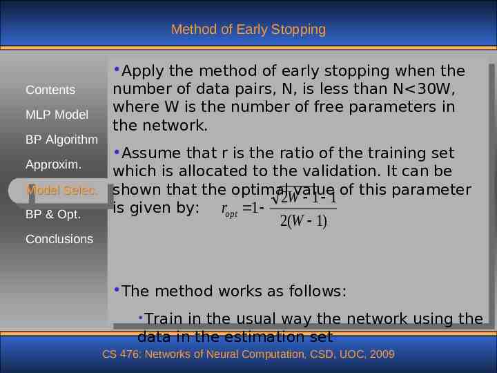
Method of Early Stopping Contents MLP Model BP Algorithm Apply the method of early stopping when the number of data pairs, N, is less than N 30W, where W is the number of free parameters in the network. Assume that r is the ratio of the training set Approxim. which is allocated to the validation. It can be Model Selec. shown that the optimal value of this parameter 2W 1 1 is given by: ropt 1 BP & Opt. 2(W 1) Conclusions The method works as follows: Train in the usual way the network using the data in the estimation set CS 476: Networks of Neural Computation, CSD, UOC, 2009
Method of Early Stopping II After Approxim. a period of estimation, the weights and bias levels of MLP are all fixed and the network is operating in its forward mode only. The validation error is measured for each example present in the validation subset Model Selec. When Contents MLP Model BP Algorithm BP & Opt. Conclusions the validation phase is completed, the estimation is resumed for another period (e.g. 10 epochs) and the process is repeated CS 476: Networks of Neural Computation, CSD, UOC, 2009
Leave k-out Validation Contents We divide the set of available examples into K subsets MLP Model The model is trained in all the subsets except BP Algorithm for one and the validation error is measured by testing it on the subset left out Approxim. Model Selec. BP & Opt. Conclusions The procedure is repeated for a total of K trials, each time using a different subset for validation The performance of the model is assessed by averaging the squared error under validation over all the trials of the experiment There is a limiting case for K N in which case the method is called leave-one-out. CS 476: Networks of Neural Computation, CSD, UOC, 2009
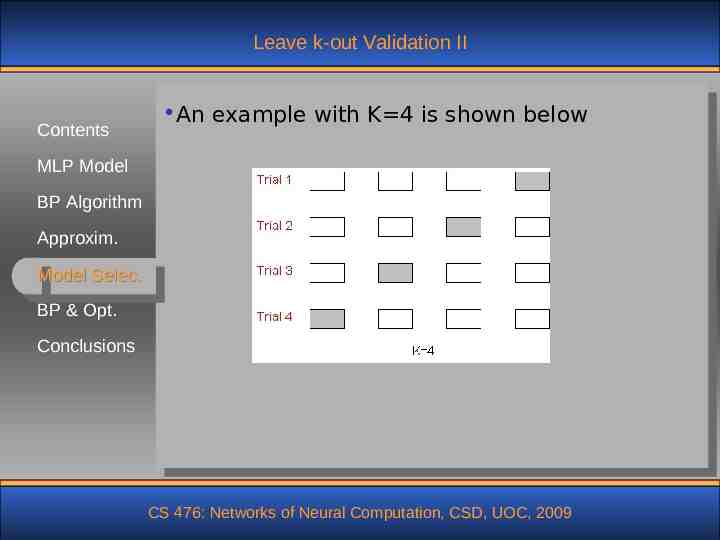
Leave k-out Validation II Contents An example with K 4 is shown below MLP Model BP Algorithm Approxim. Model Selec. BP & Opt. Conclusions CS 476: Networks of Neural Computation, CSD, UOC, 2009
Network Pruning Contents MLP Model BP Algorithm Approxim. Model Selec. BP & Opt. Conclusions To solve real world problems we need to reduce the free parameters of the model. We can achieve this objective in one of two ways: Network growing: in which case we start with a small MLP and then add a new neuron or layer of hidden neurons only when we are unable to achieve the performance level we want Network pruning: in this case we start with a large MLP with an adequate performance for the problem at hand, and then we prune it by weakening or eliminating certain weights in a principled manner CS 476: Networks of Neural Computation, CSD, UOC, 2009
Network Pruning II Contents Pruning can be implemented as a form of regularisation MLP Model BP Algorithm Approxim. Model Selec. BP & Opt. Conclusions CS 476: Networks of Neural Computation, CSD, UOC, 2009
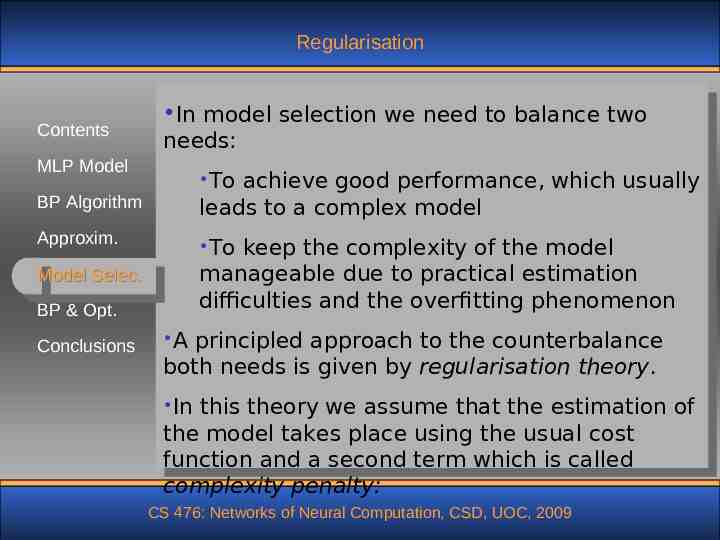
Regularisation Contents In model selection we need to balance two needs: MLP Model To achieve good performance, which usually leads to a complex model BP Algorithm Approxim. To keep the complexity of the model manageable due to practical estimation difficulties and the overfitting phenomenon Model Selec. BP & Opt. Conclusions A principled approach to the counterbalance both needs is given by regularisation theory. In this theory we assume that the estimation of the model takes place using the usual cost function and a second term which is called complexity penalty: CS 476: Networks of Neural Computation, CSD, UOC, 2009
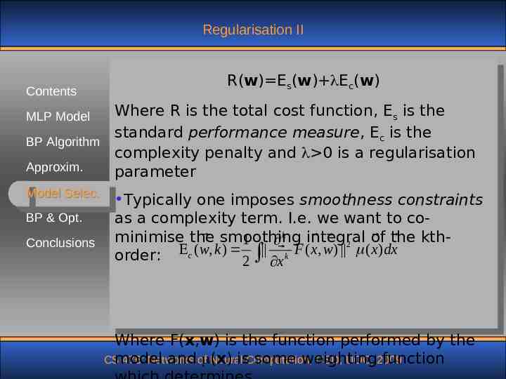
Regularisation II Contents R(w) Es(w) Ec(w) Where R is the total cost function, Es is the standard performance measure, Ec is the BP Algorithm complexity penalty and 0 is a regularisation Approxim. parameter MLP Model Model Selec. BP & Opt. Conclusions Typically one imposes smoothness constraints as a complexity term. I.e. we want to cominimise the smoothing 2 of the kth1 k integral order: c ( w, k ) 2 x k F ( x , w) ( x )dx Where F(x,w) is the function performed by the CSmodel 476: Networks Neural CSD, UOC, 2009 and of (x) isComputation, some weighting function
Regularisation III Contents the region of the input space where the function F(x,w) is required to be smooth. MLP Model BP Algorithm Approxim. Model Selec. BP & Opt. Conclusions CS 476: Networks of Neural Computation, CSD, UOC, 2009
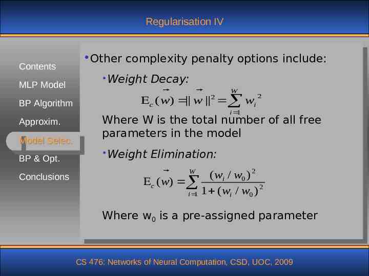
Regularisation IV Contents MLP Model BP Algorithm Other complexity penalty options include: Weight Decay: 2 W 2 c ( w) w wi i 1 Approxim. Model Selec. BP & Opt. Conclusions Where W is the total number of all free parameters in the model Weight Elimination: W ( wi / w0 ) 2 c ( w) 2 i 1 1 ( wi / w0 ) Where w0 is a pre-assigned parameter CS 476: Networks of Neural Computation, CSD, UOC, 2009
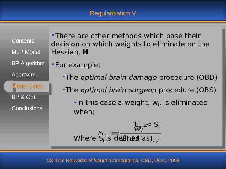
Regularisation V MLP Model There are other methods which base their decision on which weights to eliminate on the Hessian, H BP Algorithm For example: Contents Approxim. Model Selec. BP & Opt. Conclusions The optimal brain damage procedure (OBD) The optimal brain surgeon procedure (OBS) In this case a weight, wi, is eliminated when: E 2 Si wavi Si 1 Where Si is defined 2[ H as: ]i ,i CS 476: Networks of Neural Computation, CSD, UOC, 2009
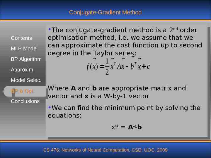
Conjugate-Gradient Method Contents MLP Model BP Algorithm Approxim. The conjugate-gradient method is a 2nd order optimisation method, i.e. we assume that we can approximate the cost function up to second degree in the Taylor series: 1 T T f ( x ) x Ax b x c 2 Model Selec. BP & Opt. Conclusions Where A and b are appropriate matrix and vector and x is a W-by-1 vector We can find the minimum point by solving the equations: x* A-1b CS 476: Networks of Neural Computation, CSD, UOC, 2009
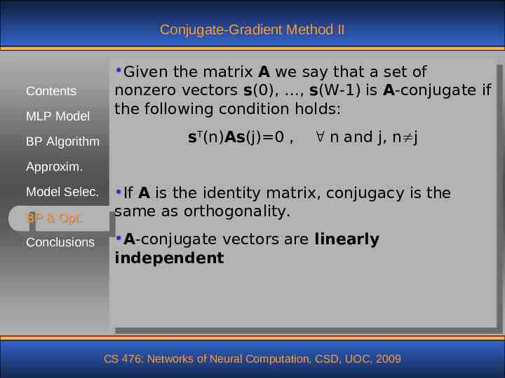
Conjugate-Gradient Method II Contents MLP Model BP Algorithm Given the matrix A we say that a set of nonzero vectors s(0), , s(W-1) is A-conjugate if the following condition holds: sT(n)As(j) 0 , n and j, n j Approxim. Model Selec. BP & Opt. Conclusions If A is the identity matrix, conjugacy is the same as orthogonality. A-conjugate vectors are linearly independent CS 476: Networks of Neural Computation, CSD, UOC, 2009
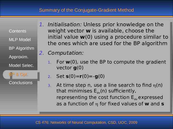
Summary of the Conjugate-Gradient Method Contents MLP Model BP Algorithm Approxim. Model Selec. BP & Opt. Conclusions 1. Initialisation: Unless prior knowledge on the weight vector w is available, choose the initial value w(0) using a procedure similar to the ones which are used for the BP algorithm 2. Computation: 1. For w(0), use the BP to compute the gradient vector g(0) 2. Set s(0) r(0) -g(0) 3. At time step n, use a line search to find (n) that minimises Eav(n) sufficiently, representing the cost function Eav expressed as a function of for fixed values of w and s CS 476: Networks of Neural Computation, CSD, UOC, 2009
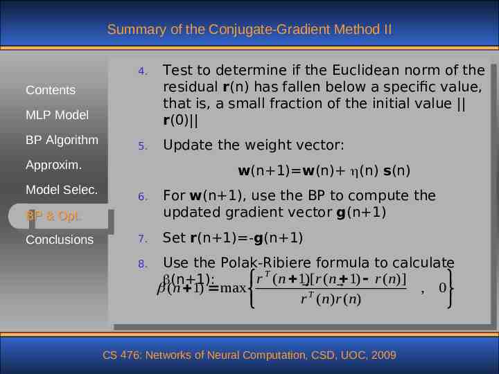
Summary of the Conjugate-Gradient Method II 4. Test to determine if the Euclidean norm of the residual r(n) has fallen below a specific value, that is, a small fraction of the initial value r(0) 5. Update the weight vector: Contents MLP Model BP Algorithm Approxim. Model Selec. w(n 1) w(n) (n) s(n) 6. For w(n 1), use the BP to compute the updated gradient vector g(n 1) 7. Set r(n 1) -g(n 1) BP & Opt. Conclusions 8. Use the Polak-Ribiere formula to T calculate r (n 1)[r (n 1) r (n)] (n 1): (n 1) max , 0 T r ( n) r ( n) CS 476: Networks of Neural Computation, CSD, UOC, 2009
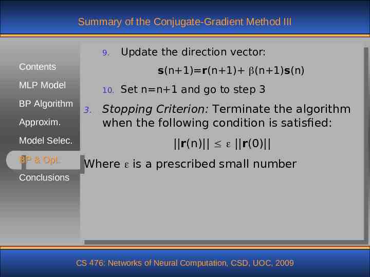
Summary of the Conjugate-Gradient Method III 9. Contents s(n 1) r(n 1) (n 1)s(n) MLP Model BP Algorithm Approxim. Model Selec. BP & Opt. Update the direction vector: 10. 3. Set n n 1 and go to step 3 Stopping Criterion: Terminate the algorithm when the following condition is satisfied: r(n) r(0) Where is a prescribed small number Conclusions CS 476: Networks of Neural Computation, CSD, UOC, 2009
Advantages & Disadvantages MLP and BP is used in Cognitive and Contents Computational Neuroscience modelling but still the algorithm does not have real neuroMLP Model physiological support BP Algorithm The algorithm can be used to make encoding / Approxim. decoding and compression systems. Useful for Model Selec. data pre-processing operations The MLP with the BP algorithm is a universal BP & Opt. approximator of functions Conclusions The algorithm is computationally efficient as it has O(W) complexity to the model parameters The algorithm has “local” robustness The convergence of the BP can be very slow, especially in large problems, depending on the CSmethod 476: Networks of Neural Computation, CSD, UOC, 2009
Advantages & Disadvantages II Contents The BP algorithm suffers from the problem of local minima MLP Model BP Algorithm Approxim. Model Selec. BP & Opt. Conclusions CS 476: Networks of Neural Computation, CSD, UOC, 2009
Types of problems The BP algorithm is used in a great variety of Contents problems: Time series predictions MLP Model Credit risk assessment BP Algorithm Pattern recognition Approxim. Speech processing Model Selec. Cognitive modelling BP & Opt. Image processing Conclusions Control Etc BP is the standard algorithm against which all other NN algorithms are compared!! CS 476: Networks of Neural Computation, CSD, UOC, 2009