Scatter-plot, Best-Fit Line, and Correlation Coefficient
16 Slides888.00 KB
Scatter-plot, Best-Fit Line, and Correlation Coefficient
Definitions: Scatter Diagrams (Scatter Plots) – a graph that shows the relationship between two quantitative variables. Explanatory Variable – predictor variable; plotted to the horizontal axis (x-axis). Response Variable – a value explained by the explanatory variable; plotted on the vertical axis (y-axis).
Why might we want to see a Scatter Plot? Statisticians and quality control technicians gather data to determine correlations (relationships) between two events (variables). Scatter plots will often show at a glance whether a relationship exists between two sets of data. It will be easy to predict a value based on a graph if there is a relationship present.
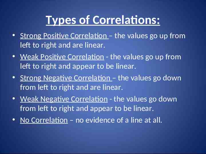
Types of Correlations: Strong Positive Correlation – the values go up from left to right and are linear. Weak Positive Correlation - the values go up from left to right and appear to be linear. Strong Negative Correlation – the values go down from left to right and are linear. Weak Negative Correlation - the values go down from left to right and appear to be linear. No Correlation – no evidence of a line at all.
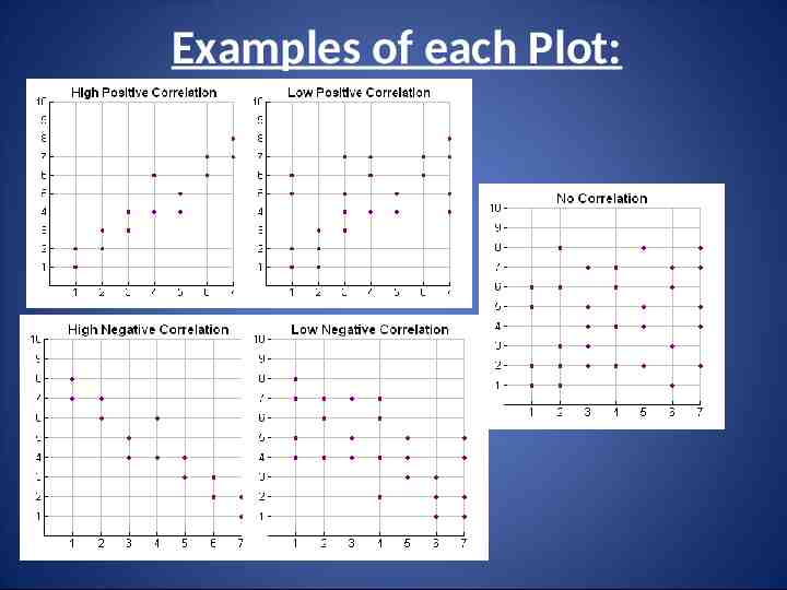
Examples of each Plot:
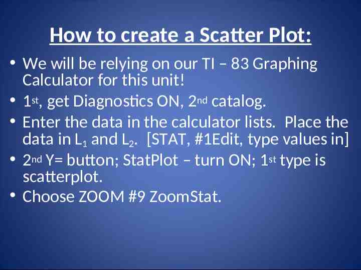
How to create a Scatter Plot: We will be relying on our TI – 83 Graphing Calculator for this unit! 1st, get Diagnostics ON, 2nd catalog. Enter the data in the calculator lists. Place the data in L1 and L2. [STAT, #1Edit, type values in] 2nd Y button; StatPlot – turn ON; 1st type is scatterplot. Choose ZOOM #9 ZoomStat.
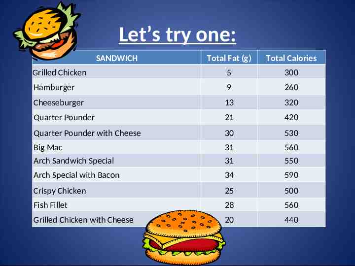
Let’s try one: SANDWICH Total Fat (g) Total Calories Grilled Chicken 5 300 Hamburger 9 260 Cheeseburger 13 320 Quarter Pounder 21 420 Quarter Pounder with Cheese 30 530 Big Mac Arch Sandwich Special 31 31 560 550 Arch Special with Bacon 34 590 Crispy Chicken 25 500 Fish Fillet 28 560 Grilled Chicken with Cheese 20 440
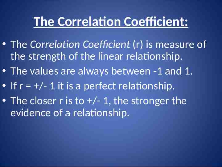
The Correlation Coefficient: The Correlation Coefficient (r) is measure of the strength of the linear relationship. The values are always between -1 and 1. If r /- 1 it is a perfect relationship. The closer r is to /- 1, the stronger the evidence of a relationship.
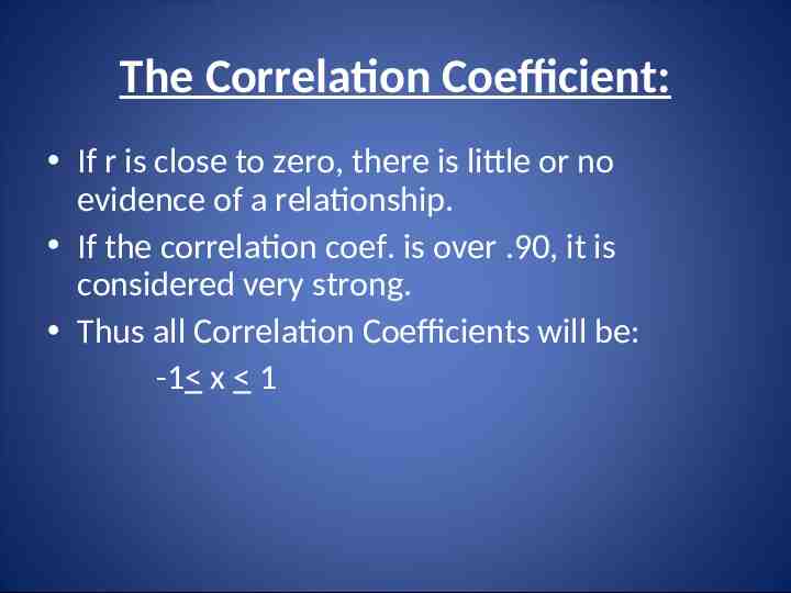
The Correlation Coefficient: If r is close to zero, there is little or no evidence of a relationship. If the correlation coef. is over .90, it is considered very strong. Thus all Correlation Coefficients will be: -1 x 1
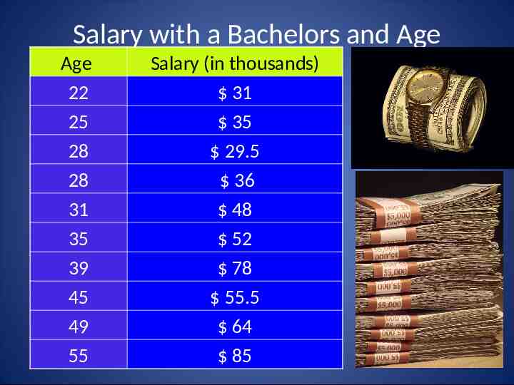
Salary with a Bachelors and Age Age 22 25 28 28 31 35 39 45 49 55 Salary (in thousands) 31 35 29.5 36 48 52 78 55.5 64 85
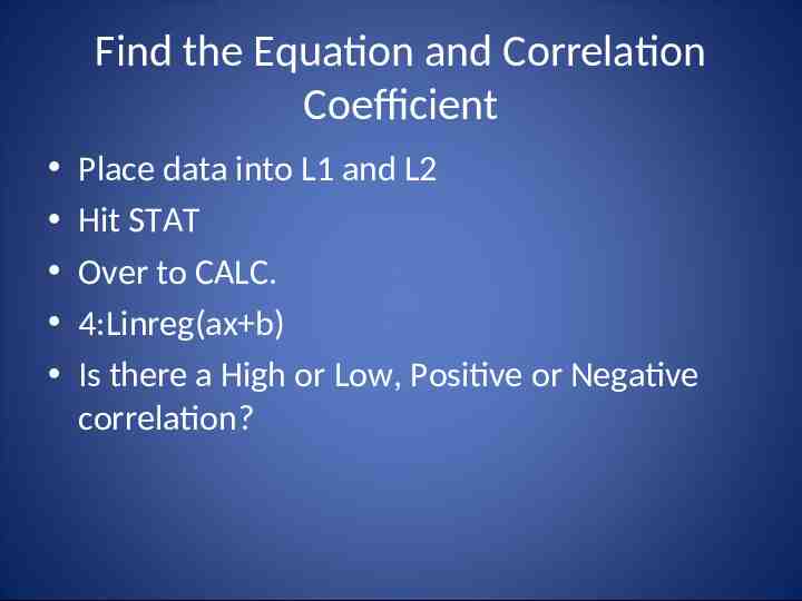
Find the Equation and Correlation Coefficient Place data into L1 and L2 Hit STAT Over to CALC. 4:Linreg(ax b) Is there a High or Low, Positive or Negative correlation?
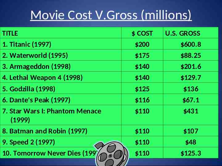
Movie Cost V.Gross (millions) TITLE COST U.S. GROSS 1. Titanic (1997) 200 600.8 2. Waterworld (1995) 175 88.25 3. Armageddon (1998) 140 201.6 4. Lethal Weapon 4 (1998) 140 129.7 5. Godzilla (1998) 125 136 6. Dante's Peak (1997) 116 67.1 7. Star Wars I: Phantom Menace (1999) 110 431 8. Batman and Robin (1997) 110 107 9. Speed 2 (1997) 110 48 10. Tomorrow Never Dies (1997) 110 125.3
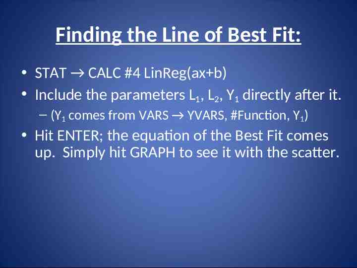
Finding the Line of Best Fit: STAT CALC #4 LinReg(ax b) Include the parameters L1, L2, Y1 directly after it. – (Y1 comes from VARS YVARS, #Function, Y1) Hit ENTER; the equation of the Best Fit comes up. Simply hit GRAPH to see it with the scatter.
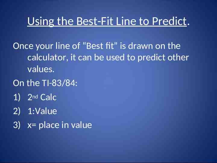
Using the Best-Fit Line to Predict. Once your line of “Best fit” is drawn on the calculator, it can be used to predict other values. On the TI-83/84: 1) 2nd Calc 2) 1:Value 3) x place in value
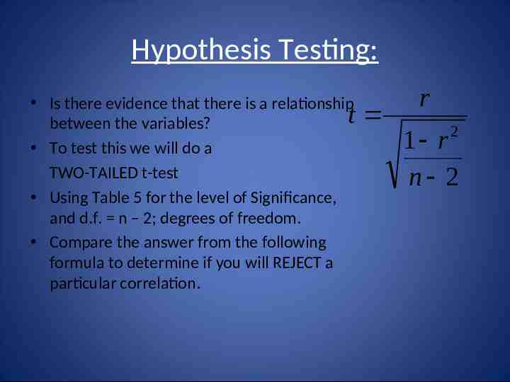
Hypothesis Testing: Is there evidence that there is a relationship t between the variables? To test this we will do a TWO-TAILED t-test Using Table 5 for the level of Significance, and d.f. n – 2; degrees of freedom. Compare the answer from the following formula to determine if you will REJECT a particular correlation. r 2 1 r n 2
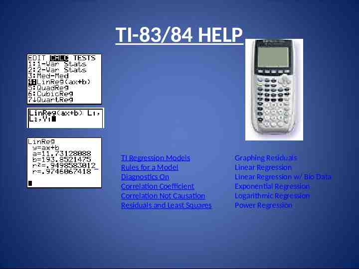
TI-83/84 HELP TI Regression Models Rules for a Model Diagnostics On Correlation Coefficient Correlation Not Causation Residuals and Least Squares Graphing Residuals Linear Regression Linear Regression w/ Bio Data Exponential Regression Logarithmic Regression Power Regression