REVIEW OF SIGNALS & SYSTEMS By: Dr. S.Chandra Mohan Reddy, Associate


90 Slides2.32 MB
REVIEW OF SIGNALS & SYSTEMS By: Dr. S.Chandra Mohan Reddy, Associate Professor and Head Department of ECE JNTUACE, Pulivendula
Introduction to Signals A Signal is a function of one or more independent variables that carries some information to represent a physical phenomenon. A continuous-time signal, also called an analog signal, is defined along a continuum of time.
A discrete-time signal is defined at discrete times.
Elementary Signals Sinusoidal & Exponential Signals Sinusoids and exponentials are important in signal and system analysis because they arise naturally in the solutions of the differential equations. Sinusoidal Signals can be expressed in either of two ways : cyclic frequency form: radian frequency form: Where and To Time Period of the Sinusoidal Wave Contd.
Sinusoidal & Exponential Signals x(t) A sin (2Пfot θ) A sin (ωot θ) x(t) Aeat Aejω̥t Sinusoidal signal Real Exponential A[cos (ωot) j sin (ωot)] Complex Exponential θ Phase of sinusoidal wave A amplitude of a sinusoidal or exponential signal fo fundamental cyclic frequency of sinusoidal signal ωo radian frequency
Unit Step Function 1 , t 0 u t 1/ 2 , t 0 0 , t 0 Precise Graph Commonly-Used Graph
Signum Function 1 , t 0 sgn t 0 , t 0 2 u t 1 1 , t 0 Precise Graph Commonly-Used Graph The signum function, is closely related to the unit-step function.
Unit Ramp Function t , t 0 t ramp t u d t u t 0 , t 0 The unit ramp function is the integral of the unit step function. It is called the unit ramp function because for positive t, its slope is one amplitude unit per time.
Rectangular Pulse or Gate Function Rectangular pulse, 1/ a , t a / 2 a t , t a/2 0
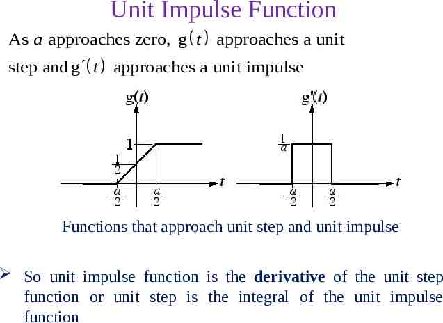
Unit Impulse Function As a approaches zero, g t approaches a unit step and g t approaches a unit impulse Functions that approach unit step and unit impulse So unit impulse function is the derivative of the unit step function or unit step is the integral of the unit impulse function
Representation of Impulse Function The area under an impulse is called its strength or weight. It is represented graphically by a vertical arrow. An impulse with a strength of one is called a unit impulse.
Properties of the Impulse Function The Sampling Property g t t t dt g t 0 0 The Scaling Property 1 a t t0 t t0 a The Replication Property g(t) δ(t) g (t)
Unit Impulse Train The unit impulse train is a sum of infinitely uniformlyspaced impulses and is given by T t t nT , n an integer n
The Unit Rectangle Function The unit rectangle or gate signal can be represented as combination of two shifted unit step signals as shown
The Unit Triangle Function A triangular pulse whose height and area are both one but its base width is not, is called unit triangle function. The unit triangle is related to the unit rectangle through an operation called convolution.
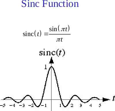
Sinc Function sinc t sin t t
Discrete-Time Signals Sampling is the acquisition of the values of a continuous-time signal at discrete points in time x(t) is a continuous-time signal, x[n] is a discretetime signal x n x nTs where Ts is the time between samples
Discrete Time Exponential and Sinusoidal Signals DT signals can be defined in a manner analogous to their continuous-time counter part x[n] A sin (2Пn/No θ) Discrete Time Sinusoidal Signal A sin (2ПFon θ) Discrete Time Exponential Signal x[n] an n the discrete time A amplitude θ phase shifting radians, No Discrete Period of the wave 1/N0 Fo Ωo/2 П Discrete Frequency
Discrete Time Sinusoidal Signals
Discrete Time Unit Step Function or Unit Sequence Function 1 , n 0 u n 0 , n 0
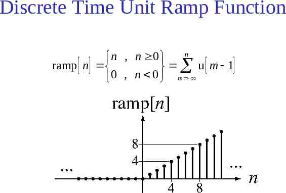
Discrete Time Unit Ramp Function n n , n 0 ramp n u m 1 0 , n 0 m
Discrete Time Unit Impulse Function or Unit Pulse Sequence 1 , n 0 n 0 , n 0 n an for any non-zero, finite integer a. Contd.
Unit Pulse Sequence The discrete-time unit impulse is a function in the ordinary sense in contrast with the continuoustime unit impulse. It has a sampling property. It has no scaling property i.e. δ[n] δ[an] for any non-zero finite integer ‘a’
Operations on Signals Sometime a given mathematical function may completely describe a signal . Different operations are required for different purposes of arbitrary signals. The operations on signals can be Time Shifting Time Scaling Time Inversion or Time Folding
Time Shifting The original signal x(t) is shifted by an amount tₒ. X(t) X(t-to) Signal Delayed Shift to the right Contd.
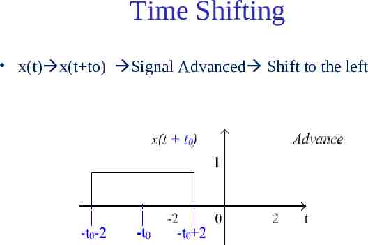
Time Shifting x(t) x(t to) Signal Advanced Shift to the left
Time Scaling For the given function x(t), x(at) is the time scaled version of x(t) For a 1,period of function x(t) reduces and function speeds up. Graph of the function shrinks. For a 1, the period of the x(t) increases and the function slows down. Graph of the function expands. Contd.
Time scaling Example: Given x(t) and we are to find y(t) x(2t). The period of x(t) is 2 and the period of y(t) is 1, Contd.
Time scaling Given y(t), – find w(t) y(3t) and v(t) y(t/3).
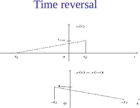
Time Reversal Time reversal is also called time folding In Time reversal signal is reversed with respect to time i.e. y(t) x(-t) is obtained for the given function Contd.
Time reversal
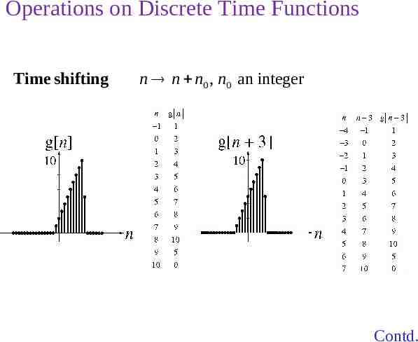
Operations on Discrete Time Functions Time shifting n n n0 , n0 an integer Contd.
Operations on Discrete Functions Scaling; Signal Compression n Kn K an integer 1
Classification of Signals Deterministic & Non Deterministic Signals Periodic & A periodic Signals Even & Odd Signals Energy & Power Signals
Deterministic & Non Deterministic Signals Deterministic signals Behavior of these signals is predictable w.r.t time There is no uncertainty with respect to its value at any time. These signals can be expressed mathematically. For example x(t) sin(3t) is deterministic signal. Contd.
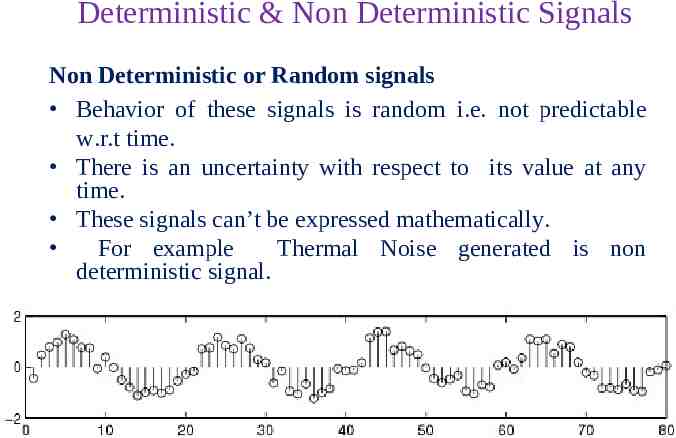
Deterministic & Non Deterministic Signals Non Deterministic or Random signals Behavior of these signals is random i.e. not predictable w.r.t time. There is an uncertainty with respect to its value at any time. These signals can’t be expressed mathematically. For example Thermal Noise generated is non deterministic signal.
Periodic and Non-periodic Signals Given x(t) is a continuous-time signal x (t) is periodic iff x(t) x(t Tₒ) for any T and any integer n Example – x(t) A cos(wt) – x(t Tₒ) A cos[w(t Tₒ)] A cos(wt wTₒ) A cos(wt 2p) A cos(wt) – Note: Tₒ 1/fₒ ; w 2pfₒ Contd.
Periodic and Non-periodic Signals For non-periodic signals x(t) x(t Tₒ) A non-periodic signal is assumed to have a period T Example of non periodic signal is an exponential signal
Important Condition of Periodicity for Discrete Time Signals A discrete time signal is periodic if x(n) x(n N) For satisfying the above condition the frequency of the discrete time signal should be ratio of two integers i.e. fₒ k/N
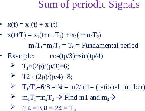
Sum of periodic Signals x(t) x1(t) x2(t) x(t T) x1(t m1T1) x2(t m2T2) m1T1 m2T2 Tₒ Fundamental period Example: cos(tp/3) sin(tp/4) T1 (2p)/(p/3) 6; T2 (2p)/(p/4) 8; T1/T2 6/8 ¾ m2/m1 (rational number) m1T1 m2T2 Find m1 and m2 6.4 3.8 24 Tₒ
Sum of periodic Signals – may not always be periodic x(t ) x1 (t ) x2 (t ) cos t sin 2t T1 (2p)/(1) 2p; T2 (2p)/(sqrt(2)); T1/T2 sqrt(2); – Note: T1/T2 sqrt(2) is an irrational number – X(t) is aperiodic
Even and Odd Signals Even Functions Odd Functions g t g t g t g t
Even and Odd Parts of Functions The even part of a function is g e t The odd part of a function is g o t g t g t 2 g t g t 2 A function whose even part is zero, is odd and a function whose odd part is zero, is even.
Various Combinations of even and odd functions Function type Sum Difference Product Quotient Both even Even Even Even Even Both odd Odd Odd Even Even Neither Odd Odd Even and odd Neither
Product of Even and Odd Functions Product of Two Even Functions Contd.
Product of Even and Odd Functions Product of an Even Function and an Odd Function Contd.
Product of Even and Odd Functions Product of an Even Function and an Odd Function Contd.
Product of Even and Odd Functions Product of Two Odd Functions
Derivatives and Integrals of Functions Function type Derivative Integral Even Odd Odd constant Odd Even Even
Discrete Time Even and Odd Signals g n g n ge n g n g n 2 g n g n g o n g n g n 2
Combination of even and odd function for DT Signals Function type Sum Difference Product Quotient Both even Even Even Even Even Both odd Odd Odd Even Even Even or odd Odd Odd Even and odd Even or Odd
Products of DT Even and Odd Functions Two Even Functions
Products of DT Even and Odd Functions An Even Function and an Odd Function Contd.
Proof Examples Prove that product of two even signals is even. x (t ) x1 (t ) x2 (t ) x ( t ) x1 ( t ) x2 ( t ) x1 (t ) x2 (t ) x(t ) Prove that product of two odd signals is odd. What is the product of an even signal and an odd signal? Prove it! Change t -t x(t ) x1 (t ) x2 (t ) x( t ) x1 ( t ) x2 ( t ) x1 (t ) x2 (t ) x(t ) x( t ) Even Contd.
Products of DT Even and Odd Functions Two Odd Functions
Energy and Power Signals Energy Signal A signal with finite energy and zero power is called Energy Signal i.e.for energy signal 0 E and P 0 Signal energy of a signal is defined as the area under the square of the magnitude of the signal. 2 Ex x t dt The units of signal energy depends on the unit of the signal. Contd.
Energy and Power Signals Power Signal Some signals have infinite signal energy. In that case it is more convenient to deal with average signal power. For power signals 0 P and E Average power of the signal Tis/ 2 given by 2 1 Px lim x t dt T T T /2 Contd.
Energy and Power Signals For a periodic signal x(t) the average signal power is 2 1 Px x t dt T T T is any period of the signal. Periodic signals are generally power signals.
Signal Energy and Power for DT Signal A discrtet time signal with finite energy and zero power is called Energy Signal i.e.for energy signal 0 E and P 0 The signal energy of a for a discrete time signal x[n] is Ex x n 2 n Contd.
Signal Energy and Power for DT Signal The average signal power of a discrete time power signal x[n] is 2 1 N 1 Px lim x n N 2N n N For a periodic signal x[n] the average signal power is 2 1 Px x n N n N The notation n N means the sum over any set of consecutive n 's exactly N in length.
What is a System? System processes input signal to produce an output signal A system is a combination of elements that manipulates one or more signals to accomplish a function to produce some output. input signal system output signal
Examples of Systems A circuit involving a capacitor can be viewed as a system that transforms the source voltage (signal) to the voltage (signal) across the capacitor A communication system is generally composed of three subsystems, the transmitter, the channel and the receiver. The channel typically attenuates and adds noise to the transmitted signal which must be processed by the receiver Biomedical system resulting in biomedical signal processing Control systems
System - Example Consider an RL series circuit R – Using a first order equation: di(t ) VL (t ) L dt di (t ) V (t ) VR VL (t ) i (t ) R L dt V(t) L
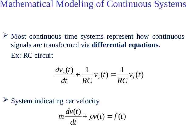
Mathematical Modeling of Continuous Systems Most continuous time systems represent how continuous signals are transformed via differential equations. Ex: RC circuit dvc (t ) 1 1 vc (t ) vs (t ) dt RC RC System indicating car velocity dv(t ) m v(t ) f (t ) dt
Mathematical Modeling of Discrete Time Systems Most discrete time systems represent how discrete signals are transformed via difference equations Ex.: Bank account, discrete car velocity system y[n] 1.01y[n 1] x[n] m v[n] v[n 1] f [ n] m m
Order of System Order of the Continuous System is the highest power of the derivative associated with the output in the differential equation dv(t ) m v(t ) f (t ) dt The order of the above system is 1. Contd.
Order of System Order of the Discrete Time system is the highest number in the difference equation by which the output is delayed y[n] 1.01y[n 1] x[n] The order of the above system is 1.
Interconnected Systems Parallel Serial (cascaded) Feedback
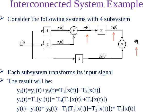
Interconnected System Example Consider the following systems with 4 subsystem Each subsystem transforms its input signal The result will be: y3(t) y1(t) y2(t) T1[x(t)] T2[x(t)] y4(t) T3[y3(t)] T3(T1[x(t)] T2[x(t)]) y(t) y4(t)* y5(t) T3(T1[x(t)] T2[x(t)])* T4[x(t)]
Feedback System Used in automatic control e(t) x(t) – y3(t) x(t) –T3[y(t)] y(t) T2[m(t)] T2(T1[e(t)]) y(t) T2(T1[x(t) – y3(t)]) T2(T1( [x(t)] –T3[y(t)] ) ) T2(T1([x(t)] –T3[y(t)]))
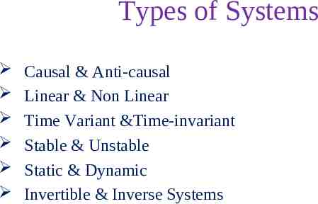
Types of Systems Causal & Anti-causal Linear & Non Linear Time Variant &Time-invariant Stable & Unstable Static & Dynamic Invertible & Inverse Systems
Causal & Anticausal Systems Causal system : A system is said to be causal if the present value of the output signal depends only on the present and/or past values of the input signal. Example: y[n] x[n] 1/2x[n-1] Anticausal system : A system is said to be anticausal if the present value of the output signal depends only on the future values of the input signal. Example: y[n] x[n 1] 1/2x[n-1]
Linear & Non Linear Systems A system is said to be linear if it satisfies the principle of superposition For checking the linearity of the given system, firstly we check the response due to linear combination of inputs Then we combine the two outputs linearly in the same manner as the inputs are combined and again total response is checked If response in step 2 and 3 are the same, the system is linear otherwise it is non linear.
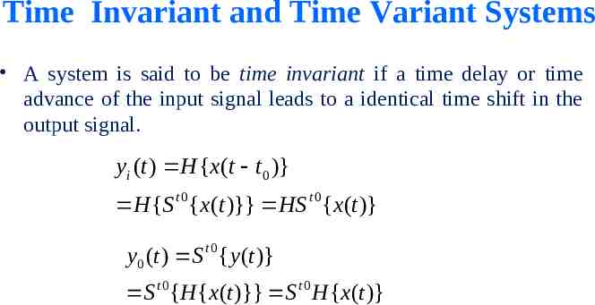
Time Invariant and Time Variant Systems A system is said to be time invariant if a time delay or time advance of the input signal leads to a identical time shift in the output signal. yi (t ) H {x(t t0 )} H {S t 0{x(t )}} HS t 0{x(t )} y0 (t ) S t 0 { y (t )} S t 0 {H {x(t )}} S t 0 H {x(t )}
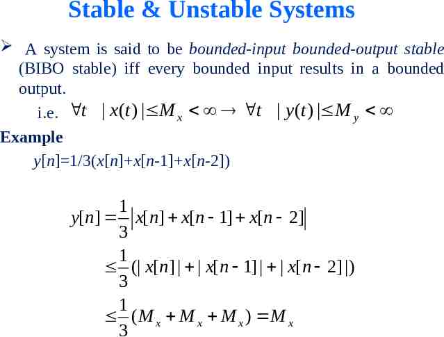
Stable & Unstable Systems A system is said to be bounded-input bounded-output stable (BIBO stable) iff every bounded input results in a bounded output. i.e. t x(t ) M x t y (t ) M y Example y[n] 1/3(x[n] x[n-1] x[n-2]) 1 y[n] x[n] x[n 1] x[n 2] 3 1 ( x[n] x[ n 1] x[ n 2] ) 3 1 ( M x M x M x ) M x 3
Stable & Unstable Systems Example: The system represented by y(t) A x(t) is unstable ; A 1 Reason: let us assume x(t) u(t), then at every instant u(t) will keep on multiplying with A and hence it will not be bounded.
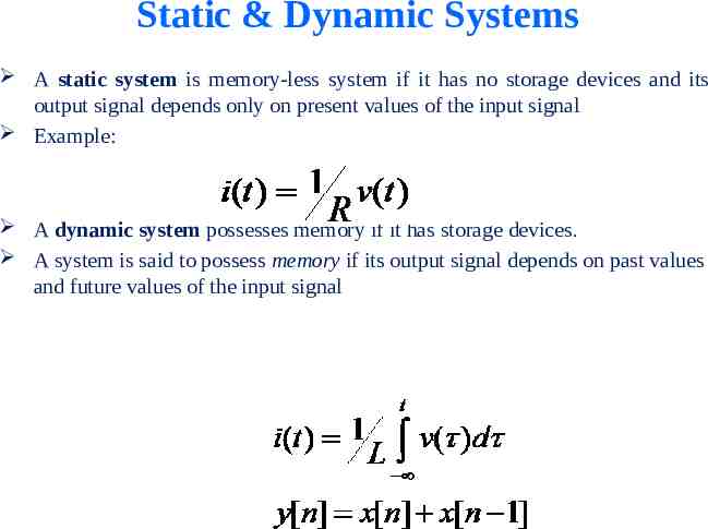
Static & Dynamic Systems A static system is memory-less system if it has no storage devices and its output signal depends only on present values of the input signal Example: A dynamic system possesses memory if it has storage devices. A system is said to possess memory if its output signal depends on past values and future values of the input signal
Invertible & Inverse Systems If a system is invertible it has an Inverse System x(t) System y(t) Inverse System x(t) Example: y(t) 2x(t) System is invertible as it has inverse system, that is: For any x(t) we get a distinct output y(t) Thus, the system must have an Inverse x(t) 1/2 y(t) z(t) x(t) System (multiplier) y(t) 2x(t) Inverse System (divider) x(t)
LTI Systems LTI Systems are completely characterized by its unit sample response The output of any LTI System is a convolution of the input signal with the unit-impulse response, i.e.
Properties of Convolution Commutative Property x[n] * h[n] h[n] * x[n] Distributive Property x[n] * (h1 [n] h2 [n]) ( x[n] * h1 [n]) ( x[n] * h2 [n]) Associative Property x[n] * h1 [n] * h2 [n] ( x[n] * h1 [n]) * h2 [n] ( x[n] * h2 [n]) * h1 [n]
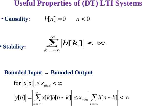
Useful Properties of (DT) LTI Systems h[n] 0 Causality: n 0 Stability: h[ k ] k Bounded Input Bounded Output for x[n] x max y[n] x[k ]h[n k ] x k max h[n k ] k
Sampling of Continuous-Time Signals Analog signals: continuous in time and amplitude Example: voltage, current, temperature, Digital signals: discrete both in time and amplitude Example: attendance of this class, digitizes analog signals, Discrete-time signal: discrete in time, continuous in amplitude Example: hourly change of temperature in Austin
Periodic (Uniform) Sampling Sampling is a continuous to discrete-time conversion -3 -2 -1 0 1 2 3 4 Most common sampling is periodic x n x c nT n T is the sampling period in second fs 1/T is the sampling frequency in Hz Sampling frequency in radian-per-second s 2 fs rad/sec This is the ideal case not the practical but close enough In practice it is implement with an analog-to-digital converters We get digital signals that are quantized in amplitude and time
Periodic Sampling Sampling is, in general, not reversible Given a sampled signal one could fit infinite continuous signals through the samples 1 0.5 0 -0.5 -1 0 20 40 60 80 100 Fundamental issue in digital signal processing If we loose information during sampling we cannot recover it Under certain conditions an analog signal can be sampled without loss so that it can be reconstructed perfectly
Representation of Sampling Mathematically convenient to represent in two stages Impulse train modulator Conversion of impulse train to a sequence s(t) xc(t) Convert impulse train to discretetime sequence x xc(t) x[n] xc(nT) x[n] s(t) -3T-2T-T 0 T 2T3T4T t -3 -2 -1 0 1 2 3 4 n
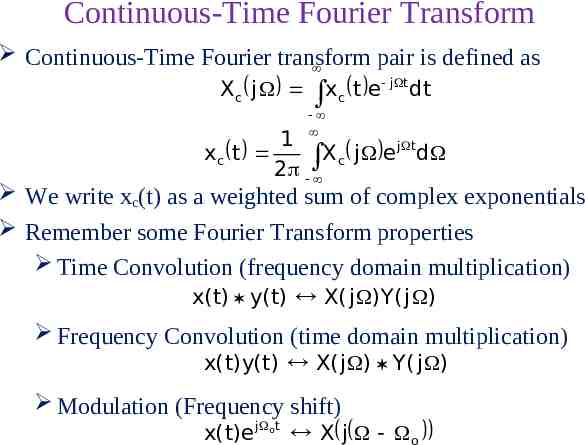
Continuous-Time Fourier Transform Continuous-Time Fourier transform pair is defined as X c j x c t e j t dt 1 j t xc t X j e d c 2 We write xc(t) as a weighted sum of complex exponentials Remember some Fourier Transform properties Time Convolution (frequency domain multiplication) x( t) y( t) X( j ) Y( j ) Frequency Convolution (time domain multiplication) x( t)y( t) X( j ) Y( j ) Modulation (Frequency shift) x( t)e j ot X j o
Frequency Domain Representation of Sampling Modulate (multiply) continuous-time signal with pulse train: x s t x c t s t x t t nT c s( t) n t nT n Let’s take the Fourier Transform of xs(t) and s(t) 1 Xs j Xc j S j 2 2 S j k s T k Fourier transform of pulse train is again a pulse train Note that multiplication in time is convolution in frequency We represent frequency with 2 f hence s 2 fs 1 X s j X c j k s T k
Frequency Domain Representation of Sampling Convolution with pulse creates replicas at pulse location: 1 X s j X c j k s T k This tells us that the impulse train modulator Creates images of the Fourier transform of the input signal Images are periodic with sampling frequency If s N sampling maybe irreversible due to aliasing of images Xc j - N N s 2 Xs j 3 s -2 s s - N N s 2 s 3 s Xs j N s 2 3 s -2 s s - N N s 2 s 3 s N
Nyquist Sampling Theorem Let xc(t) be a bandlimited signal with X c ( j ) 0 for N Then xc(t) is uniquely determined by its samples x[n] xc(nT) if s 2 2 fs 2 N T N is generally known as the Nyquist Frequency The minimum sampling rate that must be exceeded is known as the Nyquist Rate Low pass filter s 2 N Xs j 3 s -2 s s - N N s 2 s 3 s Xs j s 2 N 3 s -2 s s - N N s 2 s 3 s
THANK YOU