Reinforcement Learning Yijue Hou


34 Slides551.50 KB
Reinforcement Learning Yijue Hou
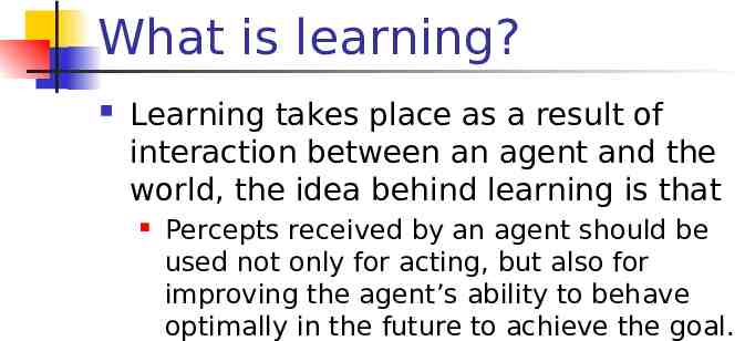
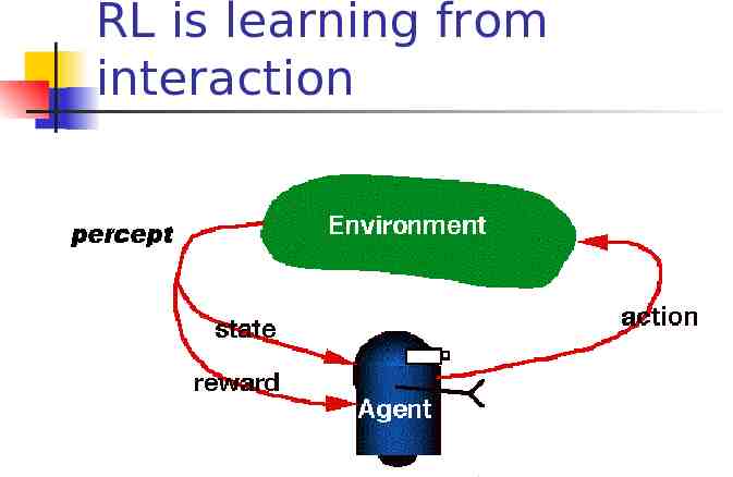
What is learning? Learning takes place as a result of interaction between an agent and the world, the idea behind learning is that Percepts received by an agent should be used not only for acting, but also for improving the agent’s ability to behave optimally in the future to achieve the goal.
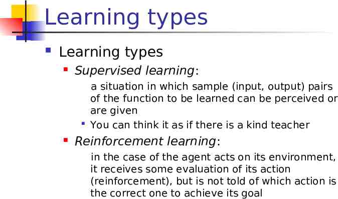
Learning types Learning types Supervised learning: a situation in which sample (input, output) pairs of the function to be learned can be perceived or are given You can think it as if there is a kind teacher Reinforcement learning: in the case of the agent acts on its environment, it receives some evaluation of its action (reinforcement), but is not told of which action is the correct one to achieve its goal
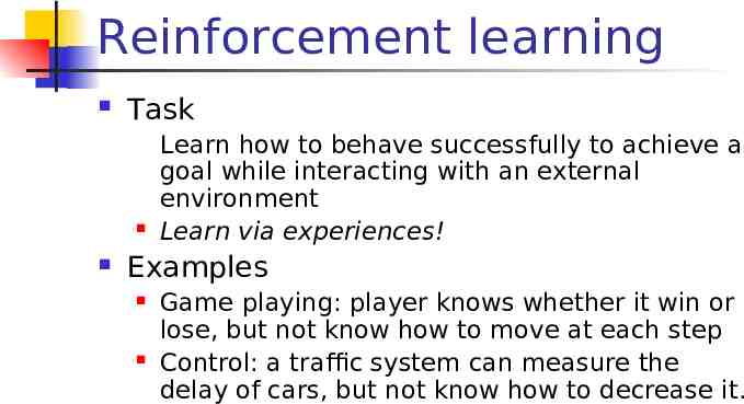
Reinforcement learning Task Learn how to behave successfully to achieve a goal while interacting with an external environment Learn via experiences! Examples Game playing: player knows whether it win or lose, but not know how to move at each step Control: a traffic system can measure the delay of cars, but not know how to decrease it.
RL is learning from interaction
RL model Each percept(e) is enough to determine the State(the state is accessible) The agent can decompose the Reward component from a percept. The agent task: to find a optimal policy, mapping states to actions, that maximize long-run measure of the reinforcement Think of reinforcement as reward Can be modeled as MDP model!
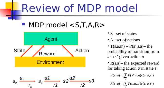
Review of MDP model MDP model S,T,A,R S– set of states Agent State Action Reward Environment s0 a0 r0 s1 a1 r1 s2 a2 r2 s3 A– set of actions T(s,a,s’) P(s’ s,a)– the probability of transition from s to s’ given action a R(s,a)– the expected reward for taking action a in state s R ( s, a ) P ( s' s, a)r ( s, a, s' ) s' R ( s, a ) T ( s, a, s ' ) r ( s, a, s ' ) s'
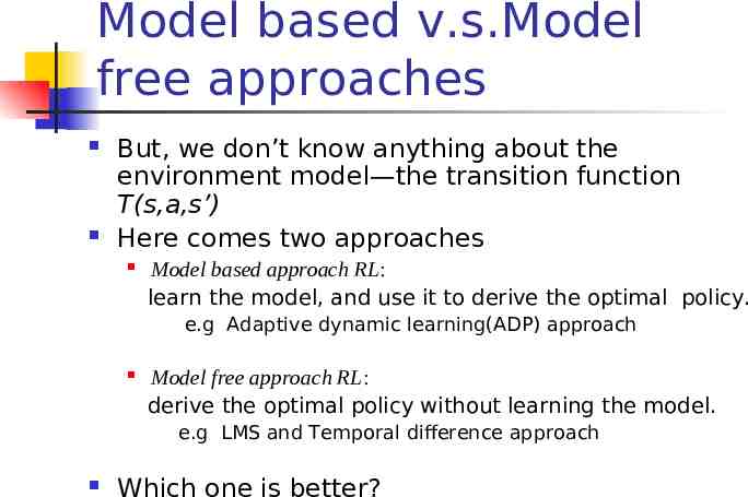
Model based v.s.Model free approaches But, we don’t know anything about the environment model—the transition function T(s,a,s’) Here comes two approaches Model based approach RL: learn the model, and use it to derive the optimal policy. e.g Adaptive dynamic learning(ADP) approach Model free approach RL: derive the optimal policy without learning the model. e.g LMS and Temporal difference approach Which one is better?
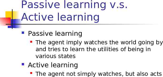
Passive learning v.s. Active learning Passive learning The agent imply watches the world going by and tries to learn the utilities of being in various states Active learning The agent not simply watches, but also acts
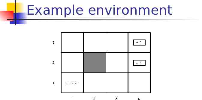
Example environment
Passive learning scenario The agent see the the sequences of state transitions and associate rewards The environment generates state transitions and the agent perceive them e.g (1,1) (1,2) (1,3) (2,3) (3,3) (4,3)[ 1] (1,1) (1,2) (1,3) (1,2) (1,3) (1,2) (1,1) (2, 1) (3,1) (4,1) (4,2)[-1] Key idea: updating the utility value using the given training sequences.
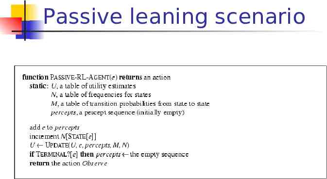
Passive leaning scenario
LMS updating Reward to go of a state the sum of the rewards from that state until a terminal state is reached Key: use observed reward to go of the state as the direct evidence of the actual expected utility of that state Learning utility function directly from sequence example
LMS updating function LMS-UPDATE (U, e, percepts, M, N ) return an updated U if TERMINAL?[e] then { reward-to-go 0 for each ei in percepts (starting from end) do s STATE[ei] reward-to-go reward-to-go REWARS[ei] U[s] RUNNING-AVERAGE (U[s], reward-to-go, N[s]) end } function RUNNING-AVERAGE (U[s], reward-to-go, N[s] ) U[s] [ U[s] * (N[s] – 1) reward-to-go ] / N[s]
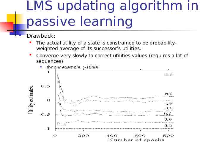
LMS updating algorithm in passive learning Drawback: The actual utility of a state is constrained to be probabilityweighted average of its successor’s utilities. Converge very slowly to correct utilities values (requires a lot of sequences) for our example, 1000!
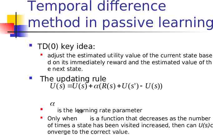
Temporal difference method in passive learning TD(0) key idea: adjust the estimated utility value of the current state base d on its immediately reward and the estimated value of th e next state. The updating rule U ( s ) U ( s ) ( R( s ) U ( s ' ) U ( s )) is the learning rate parameter Only when is a function that decreases as the number of times a state has been visited increased, then can U(s)c onverge to the correct value.
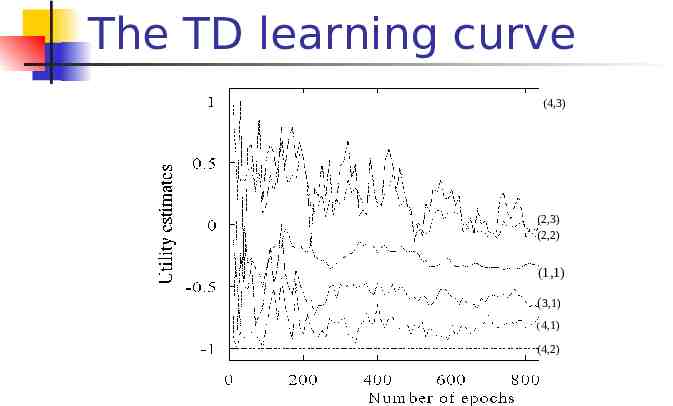
The TD learning curve (4,3) (2,3) (2,2) (1,1) (3,1) (4,1) (4,2)
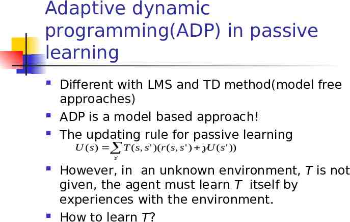
Adaptive dynamic programming(ADP) in passive learning Different with LMS and TD method(model free approaches) ADP is a model based approach! The updating rule for passive learning U ( s ) T ( s, s ' )( r ( s, s ' ) U ( s ' )) s' However, in an unknown environment, T is not given, the agent must learn T itself by experiences with the environment. How to learn T?
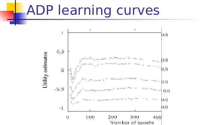
ADP learning curves (4,3) (3,3) (2,3) (1,1) (3,1) (4,1) (4,2)
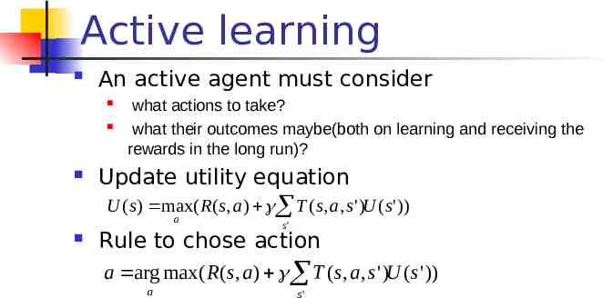
Active learning An active agent must consider what actions to take? what their outcomes maybe(both on learning and receiving the rewards in the long run)? Update utility equation U ( s) max( R( s, a ) T ( s, a, s ' )U ( s ' )) a s' Rule to chose action a arg max ( R( s, a ) T ( s, a, s ' )U ( s' )) a s'
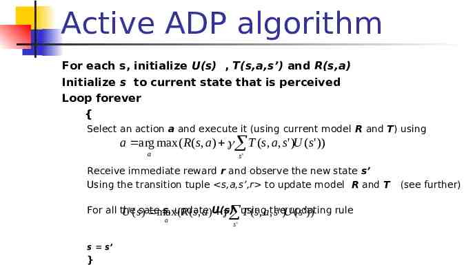
Active ADP algorithm For each s, initialize U(s) , T(s,a,s’) and R(s,a) Initialize s to current state that is perceived Loop forever { Select an action a and execute it (using current model R and T) using a arg max ( R( s, a) T ( s, a, s ' )U ( s ' )) a s' Receive immediate reward r and observe the new state s’ Using the transition tuple s,a,s’,r to update model R and T For all the s, update rule U ( ssate ) max ( R( s, a)U(s) using T ( s, a,the s ' )Uupdating ( s' )) a s s’ } s' (see further)
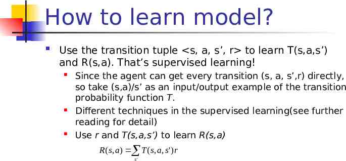
How to learn model? Use the transition tuple s, a, s’, r to learn T(s,a,s’) and R(s,a). That’s supervised learning! Since the agent can get every transition (s, a, s’,r) directly, so take (s,a)/s’ as an input/output example of the transition probability function T. Different techniques in the supervised learning(see further reading for detail) Use r and T(s,a,s’) to learn R(s,a) R( s, a ) T ( s, a, s' )r s'
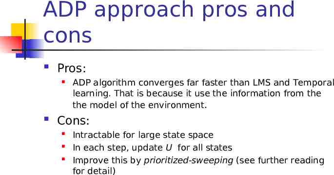
ADP approach pros and cons Pros: ADP algorithm converges far faster than LMS and Temporal learning. That is because it use the information from the the model of the environment. Cons: Intractable for large state space In each step, update U for all states Improve this by prioritized-sweeping (see further reading for detail)
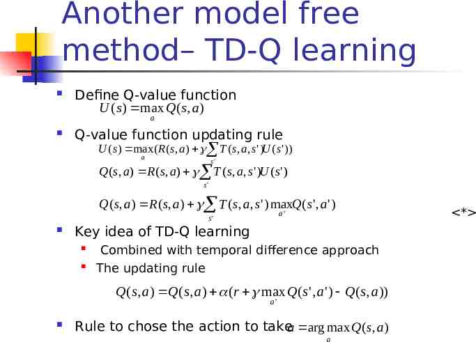
Another model free method– TD-Q learning Define Q-value function U ( s ) max Q( s, a) a Q-value function updating rule U ( s) max ( R ( s, a) T ( s, a, s ' )U ( s' )) a s' Q( s, a ) R ( s, a) T ( s, a, s ' )U ( s ' ) s' Q( s, a) R ( s, a ) T ( s, a, s ' ) maxQ( s ' , a ' ) a' s' Key idea of TD-Q learning Combined with temporal difference approach The updating rule Q( s, a) Q( s, a) (r max Q( s ' , a' ) Q( s, a)) a' Rule to chose the action to takea arg max Q( s, a) a *
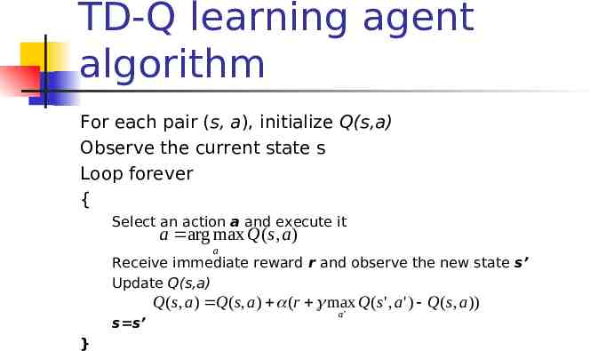
TD-Q learning agent algorithm For each pair (s, a), initialize Q(s,a) Observe the current state s Loop forever { Select an action a and execute it a arg max Q( s, a ) a Receive immediate reward r and observe the new state s’ Update Q(s,a) Q( s, a ) Q( s, a ) (r max Q( s' , a ' ) Q( s, a )) s s’ } a'
Exploration problem in Active learning An action has two kinds of outcome Gain rewards on the current experience tuple (s,a,s’) Affect the percepts received, and hence the ability of the agent to learn
Exploration problem in Active learning A trade off when choosing action between its immediately good(reflected in its current utility estimates using the what we have learned) its long term good(exploring more about the environment help it to behave optimally in the long run) Two extreme approaches “wacky”approach: acts randomly, in the hope that it will eventually explore the entire environment. “greedy”approach: acts to maximize its utility using current model estimate See Figure 20.10 Just like human in the real world! People need to decide between Continuing in a comfortable existence Or striking out into the unknown in the hopes of discovering a new and better life
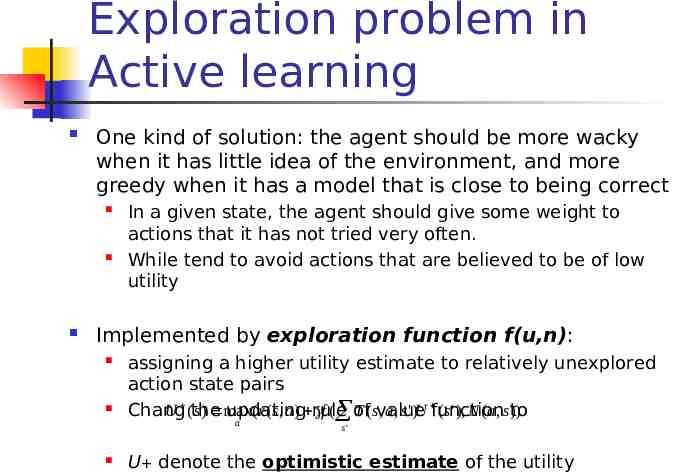
Exploration problem in Active learning One kind of solution: the agent should be more wacky when it has little idea of the environment, and more greedy when it has a model that is close to being correct In a given state, the agent should give some weight to actions that it has not tried very often. While tend to avoid actions that are believed to be of low utility Implemented by exploration function f(u,n): assigning a higher utility estimate to relatively unexplored action state pairs U (the s ) max (r ( s, a) rule f ( of T ( svalue , a, s ' )U function ( s' ), N (a, s )) Chang updating to a s' U denote the optimistic estimate of the utility
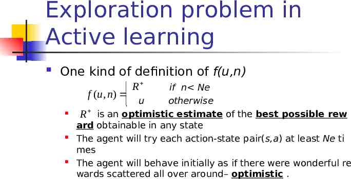
Exploration problem in Active learning One kind of definition of f(u,n) if n Ne f (u, n) u otherwise R is an optimistic estimate of the best possible rew ard obtainable in any state The agent will try each action-state pair(s,a) at least Ne ti mes The agent will behave initially as if there were wonderful re wards scattered all over around– optimistic . R
Generalization in Reinforcement Learning So far we assumed that all the functions learned by the agent are (U, T, R,Q) are tabular forms— i.e. It is possible to enumerate state and action spaces. Use generalization techniques to deal with large state or action space. Function approximation techniques
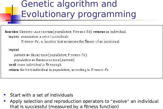
Genetic algorithm and Evolutionary programming Start with a set of individuals Apply selection and reproduction operators to “evolve” an individual that is successful (measured by a fitness function)
Genetic algorithm and Evolutionary programming Imagine the individuals as agent functions Fitness function as performance measure or reward function No attempt made to learn the relationship the rewards and actions taken by an agent Simply searches directly in the individual space to find one that maximizes the fitness functions
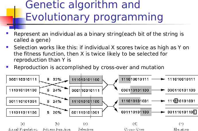
Genetic algorithm and Evolutionary programming Represent an individual as a binary string(each bit of the string is called a gene) Selection works like this: if individual X scores twice as high as Y on the fitness function, then X is twice likely to be selected for reproduction than Y is Reproduction is accomplished by cross-over and mutation
Thank you!