Reinforcement Learning I: The setting and classical stochastic dynamic
42 Slides7.30 MB
Reinforcement Learning I: The setting and classical stochastic dynamic programming algorithms Tuomas Sandholm Carnegie Mellon University Computer Science Department
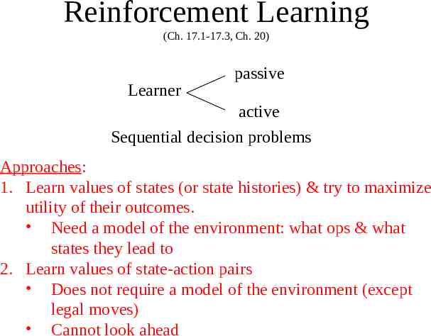
Reinforcement Learning (Ch. 17.1-17.3, Ch. 20) Learner passive active Sequential decision problems Approaches: 1. Learn values of states (or state histories) & try to maximize utility of their outcomes. Need a model of the environment: what ops & what states they lead to 2. Learn values of state-action pairs Does not require a model of the environment (except legal moves) Cannot look ahead
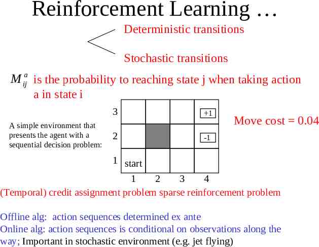
Reinforcement Learning Deterministic transitions Stochastic transitions M ija is the probability to reaching state j when taking action a in state i A simple environment that presents the agent with a sequential decision problem: 3 1 2 -1 Move cost 0.04 1 start 1 2 3 4 (Temporal) credit assignment problem sparse reinforcement problem Offline alg: action sequences determined ex ante Online alg: action sequences is conditional on observations along the way; Important in stochastic environment (e.g. jet flying)
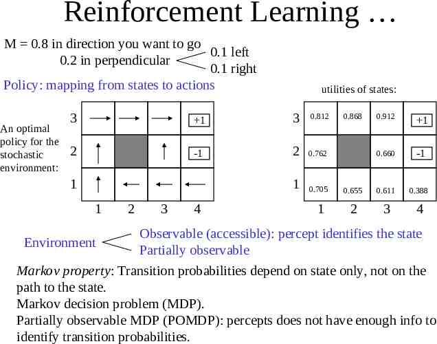
Reinforcement Learning M 0.8 in direction you want to go 0.1 left 0.2 in perpendicular 0.1 right Policy: mapping from states to actions An optimal policy for the stochastic environment: utilities of states: 3 1 3 0.812 2 -1 2 0.762 1 0.705 1 1 1 2 3 4 0.868 0.912 1 0.660 -1 0.655 0.611 0.388 2 3 4 Observable (accessible): percept identifies the state Environment Partially observable Markov property: Transition probabilities depend on state only, not on the path to the state. Markov decision problem (MDP). Partially observable MDP (POMDP): percepts does not have enough info to identify transition probabilities.
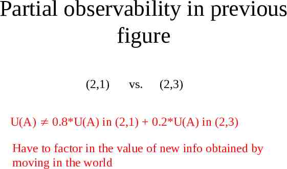
Partial observability in previous figure (2,1) vs. (2,3) U(A) 0.8*U(A) in (2,1) 0.2*U(A) in (2,3) Have to factor in the value of new info obtained by moving in the world
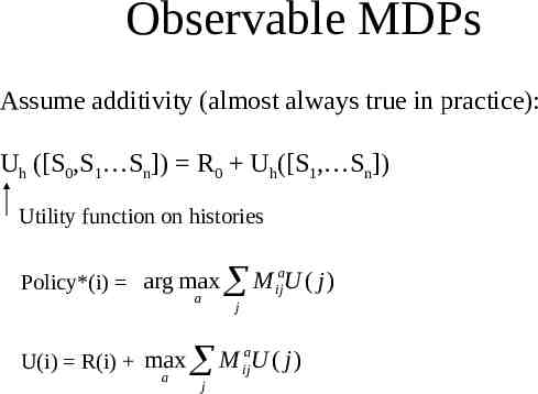
Observable MDPs Assume additivity (almost always true in practice): Uh ([S0,S1 Sn]) R0 Uh([S1, Sn]) Utility function on histories Policy*(i) arg max a U(i) R(i) max a M U ( j) j M j a ij a ij U ( j)
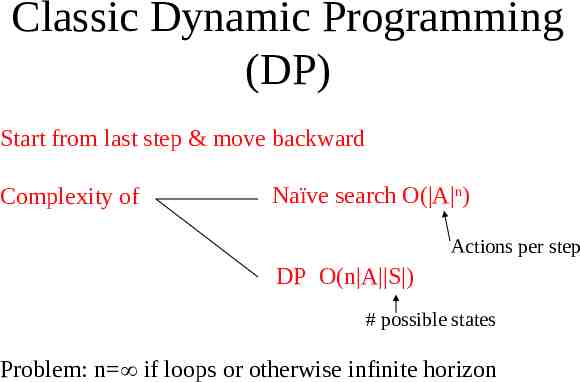
Classic Dynamic Programming (DP) Start from last step & move backward Complexity of Naïve search O( A n) Actions per step DP O(n A S ) # possible states Problem: n if loops or otherwise infinite horizon
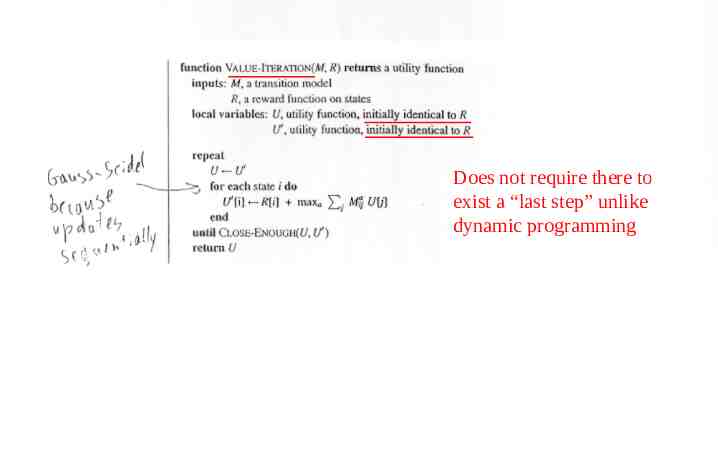
Does not require there to exist a “last step” unlike dynamic programming
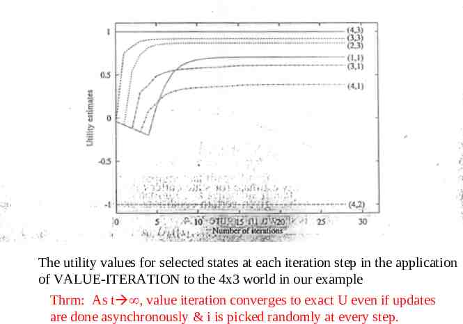
The utility values for selected states at each iteration step in the application of VALUE-ITERATION to the 4x3 world in our example Thrm: As t , value iteration converges to exact U even if updates are done asynchronously & i is picked randomly at every step.
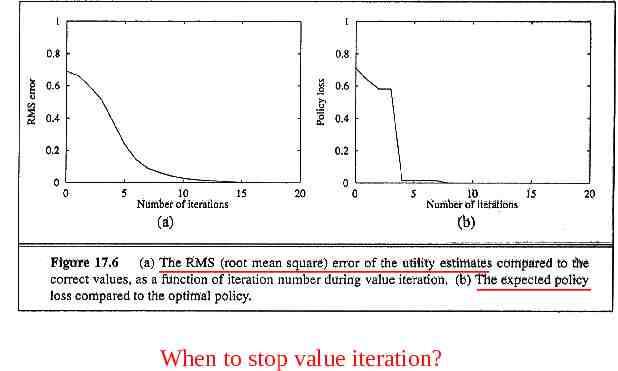
When to stop value iteration?
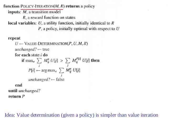
Idea: Value determination (given a policy) is simpler than value iteration
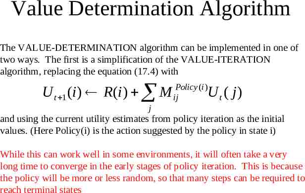
Value Determination Algorithm The VALUE-DETERMINATION algorithm can be implemented in one of two ways. The first is a simplification of the VALUE-ITERATION algorithm, replacing the equation (17.4) with U t 1 (i ) R (i ) M ijPolicy (i )U t ( j ) j and using the current utility estimates from policy iteration as the initial values. (Here Policy(i) is the action suggested by the policy in state i) While this can work well in some environments, it will often take a very long time to converge in the early stages of policy iteration. This is because the policy will be more or less random, so that many steps can be required to reach terminal states
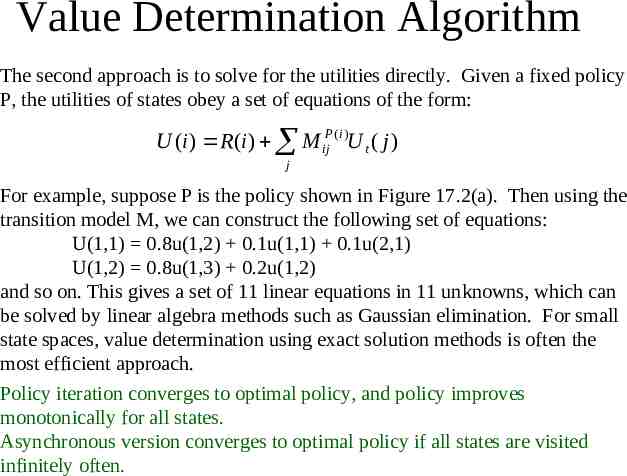
Value Determination Algorithm The second approach is to solve for the utilities directly. Given a fixed policy P, the utilities of states obey a set of equations of the form: U (i ) R (i ) M ijP (i )U t ( j ) j For example, suppose P is the policy shown in Figure 17.2(a). Then using the transition model M, we can construct the following set of equations: U(1,1) 0.8u(1,2) 0.1u(1,1) 0.1u(2,1) U(1,2) 0.8u(1,3) 0.2u(1,2) and so on. This gives a set of 11 linear equations in 11 unknowns, which can be solved by linear algebra methods such as Gaussian elimination. For small state spaces, value determination using exact solution methods is often the most efficient approach. Policy iteration converges to optimal policy, and policy improves monotonically for all states. Asynchronous version converges to optimal policy if all states are visited infinitely often.
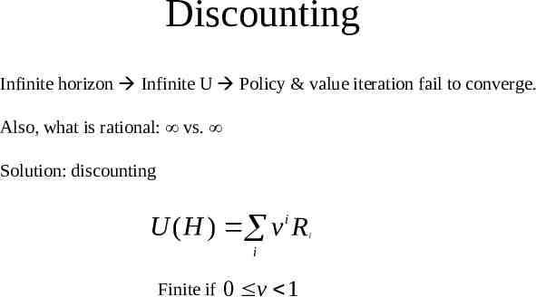
Discounting Infinite horizon Infinite U Policy & value iteration fail to converge. Also, what is rational: vs. Solution: discounting U ( H ) v i R i Finite if 0 v 1 i
Reinforcement Learning II: Reinforcement learning (RL) algorithms (we will focus solely on observable environments in this lecture) Tuomas Sandholm Carnegie Mellon University Computer Science Department
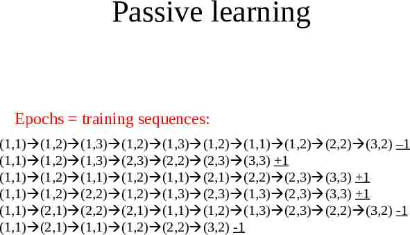
Passive learning Epochs training sequences: (1,1) (1,2) (1,3) (1,2) (1,3) (1,2) (1,1) (1,2) (2,2) (3,2) –1 (1,1) (1,2) (1,3) (2,3) (2,2) (2,3) (3,3) 1 (1,1) (1,2) (1,1) (1,2) (1,1) (2,1) (2,2) (2,3) (3,3) 1 (1,1) (1,2) (2,2) (1,2) (1,3) (2,3) (1,3) (2,3) (3,3) 1 (1,1) (2,1) (2,2) (2,1) (1,1) (1,2) (1,3) (2,3) (2,2) (3,2) -1 (1,1) (2,1) (1,1) (1,2) (2,2) (3,2) -1
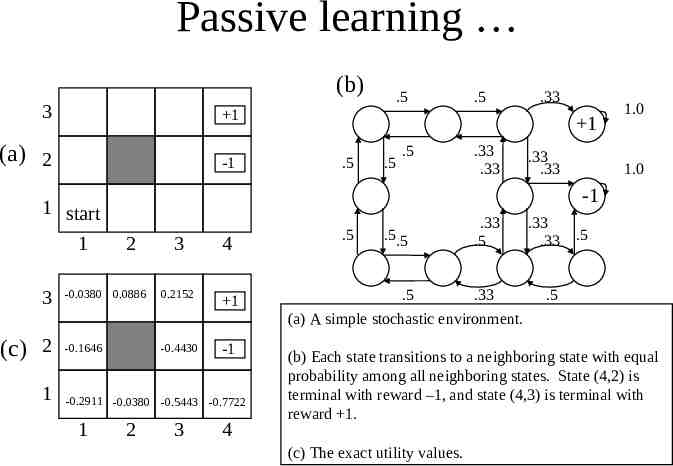
Passive learning (b) 3 1 (a) 2 -1 1 start 1 3 (c) 2 1 .5 .33 1 .5 .5 .5 .33 .33 .33 .33 1.0 1.0 -1 3 4 -0.0380 0.0886 0.2152 1 -0.1646 -0.4430 -1 2 -0.2911 -0.0380 -0.5443 -0.7722 1 .5 2 3 4 .5 .5.5 .33 .5 .5 .33 (a) A simple stochastic environment. .33 .33 .5 .5 (b) Each state transitions to a neighboring state with equal probability among all neighboring states. State (4,2) is terminal with reward –1, and state (4,3) is terminal with reward 1. (c) The exact utility values.
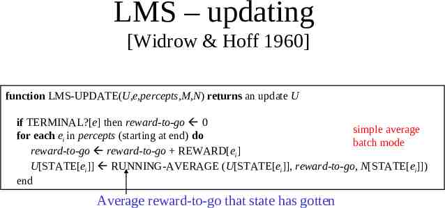
LMS – updating [Widrow & Hoff 1960] function LMS-UPDATE(U,e,percepts,M,N) returns an update U if TERMINAL?[e] then reward-to-go 0 simple average for each ei in percepts (starting at end) do batch mode reward-to-go reward-to-go REWARD[ei] U[STATE[ei]] RUNNING-AVERAGE (U[STATE[ei]], reward-to-go, N[STATE[ei]]) end Average reward-to-go that state has gotten
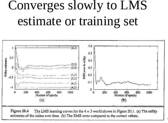
Converges slowly to LMS estimate or training set
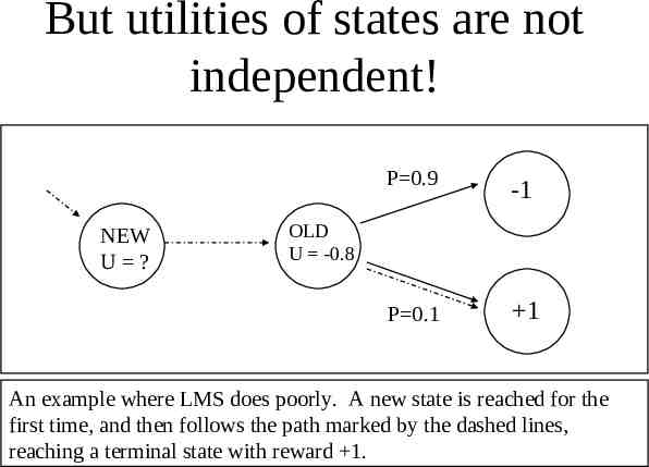
But utilities of states are not independent! NEW U ? P 0.9 -1 P 0.1 1 OLD U -0.8 An example where LMS does poorly. A new state is reached for the first time, and then follows the path marked by the dashed lines, reaching a terminal state with reward 1.
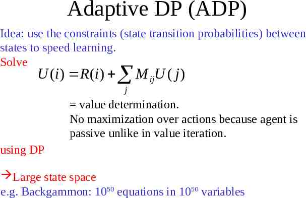
Adaptive DP (ADP) Idea: use the constraints (state transition probabilities) between states to speed learning. Solve U (i ) R (i ) M ijU ( j ) j value determination. No maximization over actions because agent is passive unlike in value iteration. using DP Large state space e.g. Backgammon: 1050 equations in 1050 variables
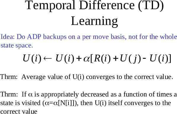
Temporal Difference (TD) Learning Idea: Do ADP backups on a per move basis, not for the whole state space. U (i ) U (i ) [ R (i ) U ( j ) U (i )] Thrm: Average value of U(i) converges to the correct value. Thrm: If is appropriately decreased as a function of times a state is visited ( [N[i]]), then U(i) itself converges to the correct value
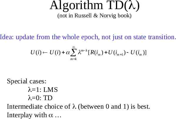
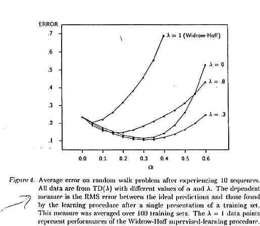
Algorithm TD( ) (not in Russell & Norvig book) Idea: update from the whole epoch, not just on state transition. U (i ) U (i ) m k [ R (im ) U (im 1 ) U (im )] m k Special cases: 1: LMS 0: TD Intermediate choice of (between 0 and 1) is best. Interplay with
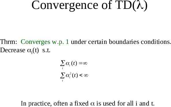
Convergence of TD( ) Thrm: Converges w.p. 1 under certain boundaries conditions. Decrease i(t) s.t. i (t ) t i2 (t ) t In practice, often a fixed is used for all i and t.
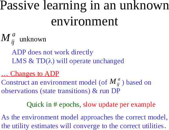
Passive learning in an unknown environment M a ij unknown ADP does not work directly LMS & TD( ) will operate unchanged Changes to ADP a M Construct an environment model (of ij ) based on observations (state transitions) & run DP Quick in # epochs, slow update per example As the environment model approaches the correct model, the utility estimates will converge to the correct utilities.
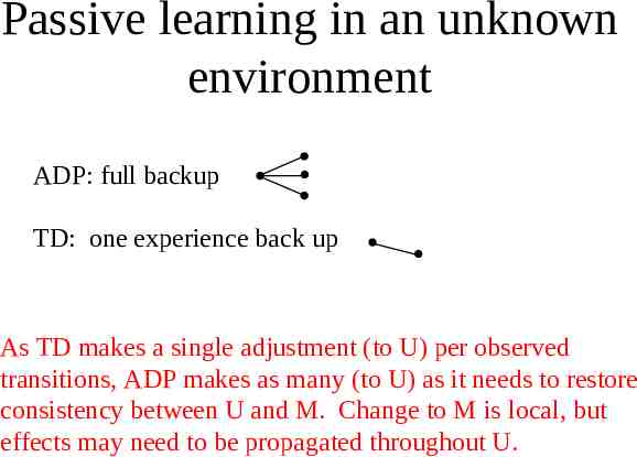
Passive learning in an unknown environment ADP: full backup TD: one experience back up As TD makes a single adjustment (to U) per observed transitions, ADP makes as many (to U) as it needs to restore consistency between U and M. Change to M is local, but effects may need to be propagated throughout U.
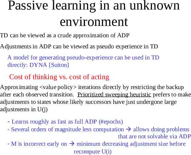
Passive learning in an unknown environment TD can be viewed as a crude approximation of ADP Adjustments in ADP can be viewed as pseudo experience in TD A model for generating pseudo-experience can be used in TD directly: DYNA [Sutton] Cost of thinking vs. cost of acting Approximating value policy iterations directly by restricting the backup after each observed transition. Prioritized sweeping heuristic prefers to make adjustments to states whose likely successors have just undergone large adjustments in U(j) - Learns roughly as fast as full ADP (#epochs) - Several orders of magnitude less computation allows doing problems that are not solvable via ADP - M is incorrect early on minimum decreasing adjustment size before recompute U(i)
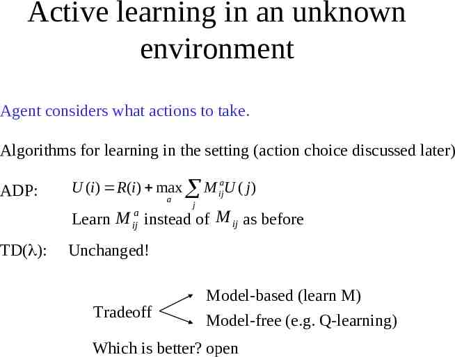
Active learning in an unknown environment Agent considers what actions to take. Algorithms for learning in the setting (action choice discussed later) ADP: U (i ) R(i ) max M ijaU ( j ) a j Learn M instead of M ij as before a ij TD( ): Unchanged! Tradeoff Model-based (learn M) Model-free (e.g. Q-learning) Which is better? open
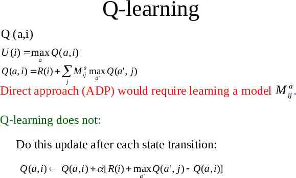
Q-learning Q (a,i) U (i ) max Q(a, i) a Q(a, i ) R (i ) M ija max Q(a' , j ) j a' Direct approach (ADP) would require learning a model M ija . Q-learning does not: Do this update after each state transition: Q(a, i ) Q(a, i ) [ R (i ) max Q(a ' , j ) Q(a, i )] a'
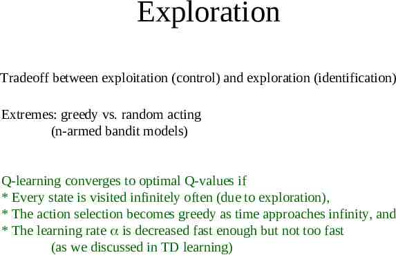
Exploration Tradeoff between exploitation (control) and exploration (identification) Extremes: greedy vs. random acting (n-armed bandit models) Q-learning converges to optimal Q-values if * Every state is visited infinitely often (due to exploration), * The action selection becomes greedy as time approaches infinity, and * The learning rate is decreased fast enough but not too fast (as we discussed in TD learning)
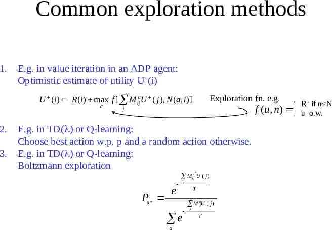
Common exploration methods 1. E.g. in value iteration in an ADP agent: Optimistic estimate of utility U (i) Exploration fn. e.g. U (i ) R(i ) max f [ M ijaU ( j ), N (a, i )] a 2. 3. f (u , n) j E.g. in TD( ) or Q-learning: Choose best action w.p. p and a random action otherwise. E.g. in TD( ) or Q-learning: Boltzmann exploration * M ija U ( j ) Pa* e j T M ijaU ( j ) e a j T R if n N u o.w.
Reinforcement Learning III: Advanced topics Tuomas Sandholm Carnegie Mellon University Computer Science Department
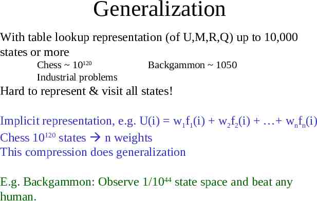
Generalization With table lookup representation (of U,M,R,Q) up to 10,000 states or more Chess 10120 Industrial problems Backgammon 1050 Hard to represent & visit all states! Implicit representation, e.g. U(i) w1f1(i) w2f2(i) wnfn(i) Chess 10120 states n weights This compression does generalization E.g. Backgammon: Observe 1/1044 state space and beat any human.
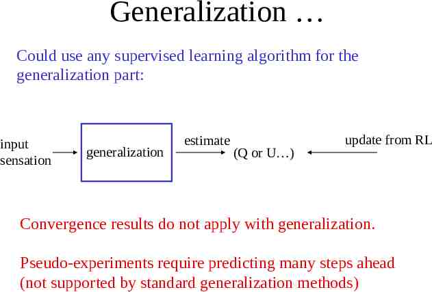
Generalization Could use any supervised learning algorithm for the generalization part: input sensation generalization estimate (Q or U ) update from RL Convergence results do not apply with generalization. Pseudo-experiments require predicting many steps ahead (not supported by standard generalization methods)
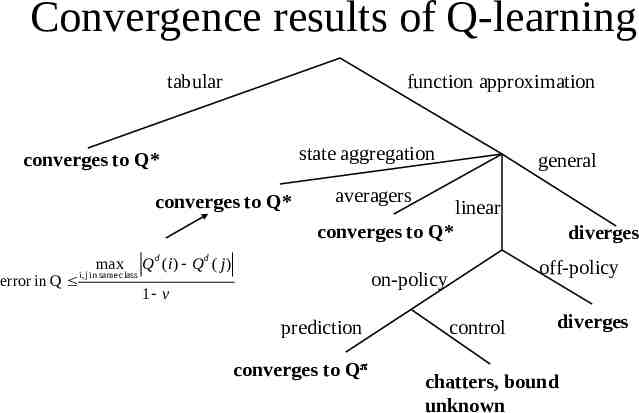
Convergence results of Q-learning tabular function approximation state aggregation converges to Q* converges to Q* general averagers linear converges to Q* error in Q max i, j in same class Q d (i ) Q d ( j ) off-policy on-policy 1 v prediction converges to Q diverges control diverges chatters, bound unknown
Applications of RL Checker’s [Samuel 59] TD-Gammon [Tesauro 92] World’s best downpeak elevator dispatcher [Crites at al 95] Inventory management [Bertsekas et al 95] – 10-15% better than industry standard Dynamic channel assignment [Singh & Bertsekas, Nie&Haykin 95] – Outperforms best heuristics in the literature Cart-pole [Michie&Chambers 68-] with bang-bang control Robotic manipulation [Grupen et al. 93-] Path planning Robot docking [Lin 93] Parking Football Tetris Multiagent RL [Tan 93, Sandholm&Crites 95, Sen 94-, Carmel&Markovitch 95-, lots of work since] Combinatorial optimization: maintenance & repair – Control of reasoning [Zhang & Dietterich IJCAI-95]
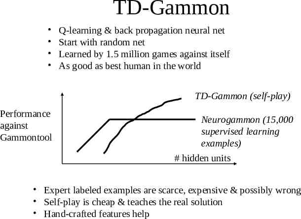
TD-Gammon Q-learning & back propagation neural net Start with random net Learned by 1.5 million games against itself As good as best human in the world TD-Gammon (self-play) Performance against Gammontool Neurogammon (15,000 supervised learning examples) # hidden units Expert labeled examples are scarce, expensive & possibly wrong Self-play is cheap & teaches the real solution Hand-crafted features help
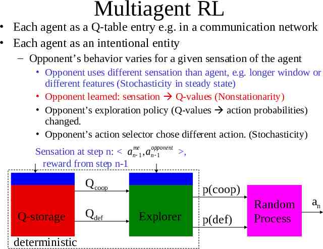
Multiagent RL Each agent as a Q-table entry e.g. in a communication network Each agent as an intentional entity – Opponent’s behavior varies for a given sensation of the agent Opponent uses different sensation than agent, e.g. longer window or different features (Stochasticity in steady state) Opponent learned: sensation Q-values (Nonstationarity) Opponent’s exploration policy (Q-values action probabilities) changed. Opponent’s action selector chose different action. (Stochasticity) Sensation at step n: anme 1 , anopponent , 1 reward from step n-1 Qcoop Q-storage deterministic Qdef p(coop) Explorer p(def) Random Process an
Future research in RL Function approximation (& convergence results) On-line experience vs. simulated experience Amount of search in action selection Exploration method (safe?) Kind of backups – Full (DP) vs. sample backups (TD) – Shallow (Monte Carlo) vs. deep (exhaustive) controls this in TD( ) Macros – Advantages Reduce complexity of learning by learning subgoals (macros) first Can be learned by TD( ) – Problems Selection of macro action Learn models of macro actions (predict their outcome) How do you come up with subgoals