Introduction to Logistic Regression Rachid Salmi,


38 Slides507.50 KB
Introduction to Logistic Regression Rachid Salmi, Jean-Claude Desenclos, Thomas Grein, Alain Moren
Oral contraceptives (OC) and myocardial infarction (MI) Case-control study, unstratified data OC MI Yes No 693 307 320 680 1000 1000 Total Controls OR 4.8 Ref.
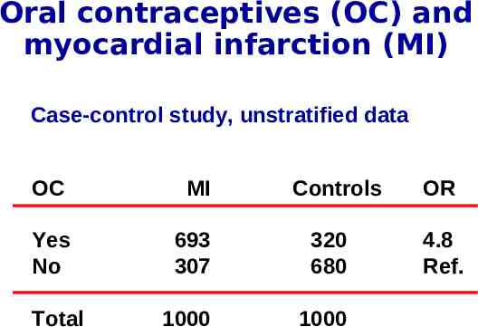
Oral contraceptives (OC) and myocardial infarction (MI) Case-control study, unstratified data Smoking Yes No Total MI Controls 700 300 500 500 1000 1000 OR 2.3 Ref.
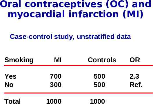
Odds ratio for OC adjusted for smoking 4 .5
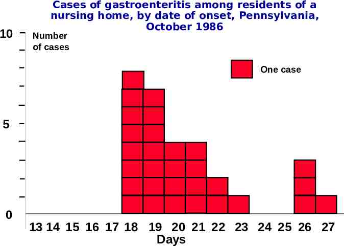
10 Cases of gastroenteritis among residents of a nursing home, by date of onset, Pennsylvania, October 1986 Number of cases One case 5 0 13 14 15 16 17 18 19 20 21 22 23 24 25 26 27 Days
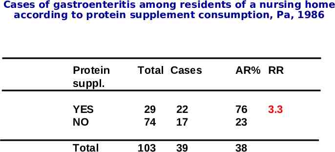
Cases of gastroenteritis among residents of a nursing home according to protein supplement consumption, Pa, 1986 Protein suppl. Total Cases AR% RR YES NO 29 74 22 17 76 23 Total 103 39 38 3.3
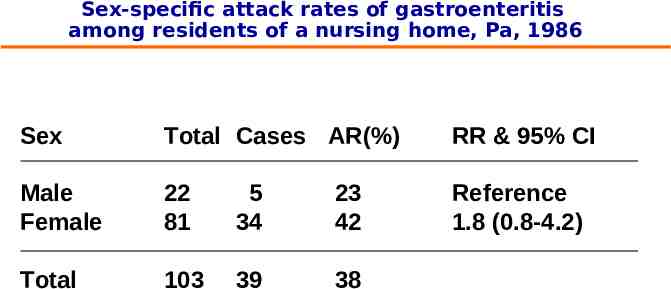
Sex-specific attack rates of gastroenteritis among residents of a nursing home, Pa, 1986 Sex Total Cases AR(%) RR & 95% CI Male Female 22 81 5 34 23 42 Reference 1.8 (0.8-4.2) Total 103 39 38
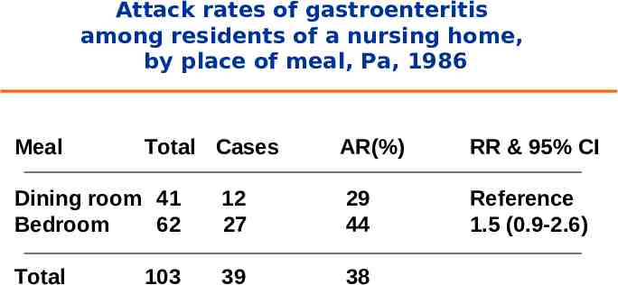
Attack rates of gastroenteritis among residents of a nursing home, by place of meal, Pa, 1986 Meal Total Cases AR(%) RR & 95% CI Reference 1.5 (0.9-2.6) Dining room 41 Bedroom 62 12 27 29 44 Total 39 38 103
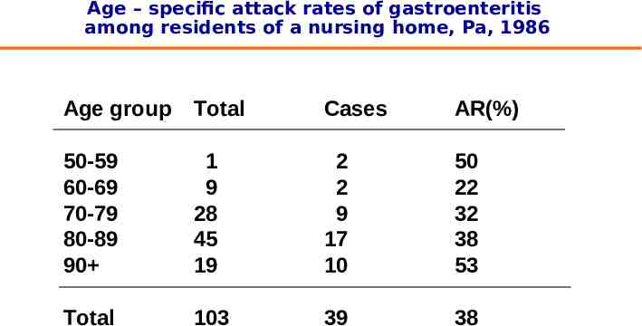
Age – specific attack rates of gastroenteritis among residents of a nursing home, Pa, 1986 Age group Total Cases AR(%) 50-59 60-69 70-79 80-89 90 1 9 28 45 19 2 2 9 17 10 50 22 32 38 53 Total 103 39 38
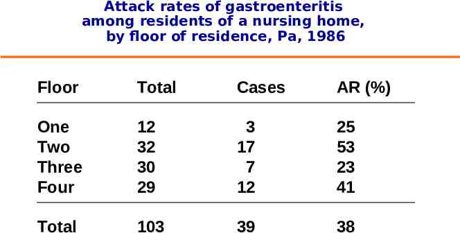
Attack rates of gastroenteritis among residents of a nursing home, by floor of residence, Pa, 1986 Floor Total Cases AR (%) One Two Three Four 12 32 30 29 3 17 7 12 25 53 23 41 Total 103 39 38
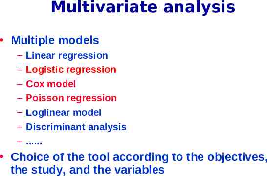
Multivariate analysis Multiple models – – – – – – – Linear regression Logistic regression Cox model Poisson regression Loglinear model Discriminant analysis . Choice of the tool according to the objectives, the study, and the variables
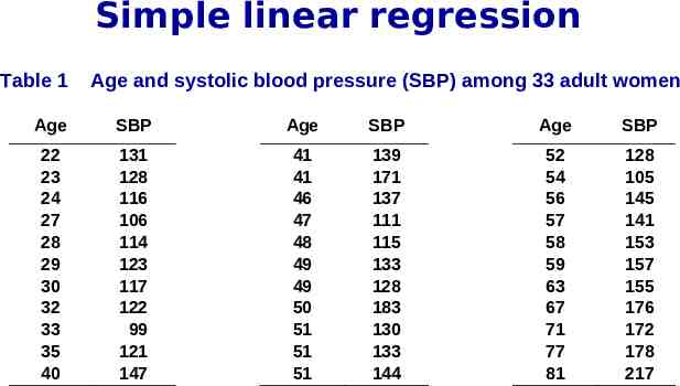
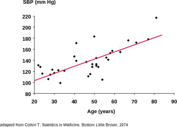
Simple linear regression Table 1 Age and systolic blood pressure (SBP) among 33 adult women Age SBP Age SBP Age SBP 22 23 24 27 28 29 30 32 33 35 40 131 128 116 106 114 123 117 122 99 121 147 41 41 46 47 48 49 49 50 51 51 51 139 171 137 111 115 133 128 183 130 133 144 52 54 56 57 58 59 63 67 71 77 81 128 105 145 141 153 157 155 176 172 178 217
SBP (mm Hg) 220 200 180 160 140 120 100 80 20 30 40 50 60 Age (years) adapted from Colton T. Statistics in Medicine. Boston: Little Brown, 1974 70 80 90
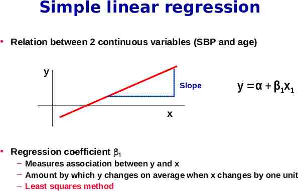
Simple linear regression Relation between 2 continuous variables (SBP and age) y Slope y α β1x 1 x Regression coefficient 1 – Measures association between y and x – Amount by which y changes on average when x changes by one unit – Least squares method
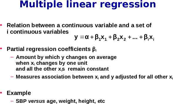
Multiple linear regression Relation between a continuous variable and a set of i continuous variables y α β1x 1 β 2 x 2 . βi x i Partial regression coefficients i – Amount by which y changes on average when xi changes by one unit and all the other xis remain constant – Measures association between xi and y adjusted for all other xi Example – SBP versus age, weight, height, etc
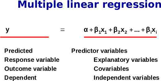
Multiple linear regression y Predicted Response variable Outcome variable Dependent α β1x 1 β 2 x 2 . βi x i Predictor variables Explanatory variables Covariables Independent variables
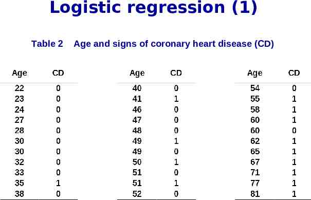
Logistic regression (1) Table 2 Age and signs of coronary heart disease (CD)
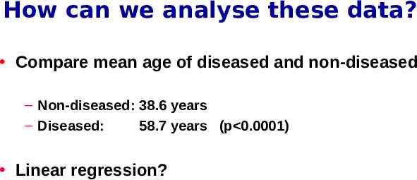
How can we analyse these data? Compare mean age of diseased and non-diseased – Non-diseased: 38.6 years – Diseased: 58.7 years (p 0.0001) Linear regression?
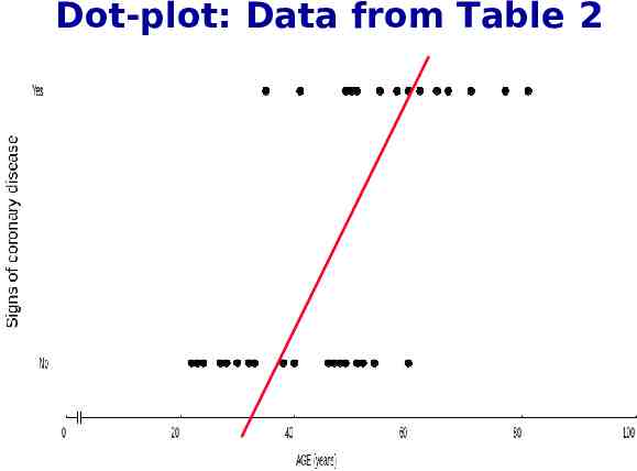
Dot-plot: Data from Table 2
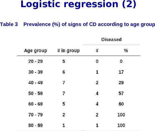
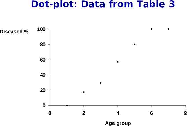
Logistic regression (2) Table 3 Prevalence (%) of signs of CD according to age group
Dot-plot: Data from Table 3 Diseased % 100 80 60 40 20 0 0 2 4 Age group 6 8
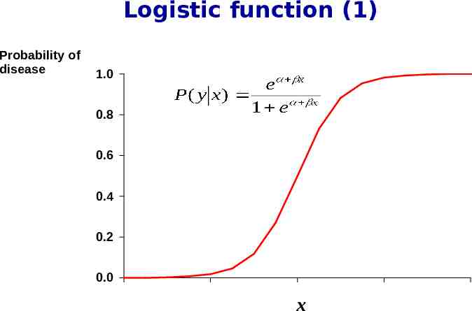
Logistic function (1) Probability of disease 1.0 0.8 0.6 0.4 0.2 0.0 x
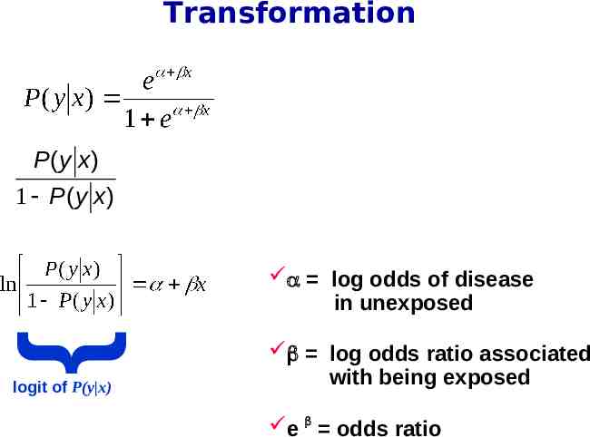
Transformation P(y x) 1 P(y x) { log odds of disease in unexposed logit of P(y x) log odds ratio associated with being exposed e odds ratio
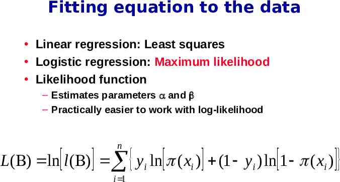
Fitting equation to the data Linear regression: Least squares Logistic regression: Maximum likelihood Likelihood function – Estimates parameters and – Practically easier to work with log-likelihood n L( ) ln l ( ) yi ln ( xi ) (1 yi ) ln 1 ( xi ) i 1
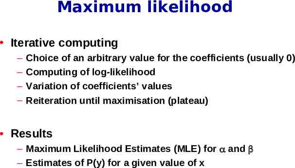
Maximum likelihood Iterative computing – – – – Choice of an arbitrary value for the coefficients (usually 0) Computing of log-likelihood Variation of coefficients’ values Reiteration until maximisation (plateau) Results – Maximum Likelihood Estimates (MLE) for and – Estimates of P(y) for a given value of x
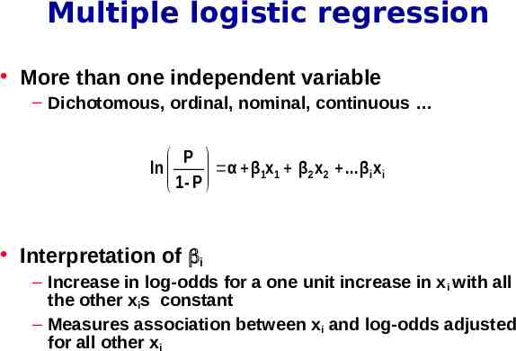
Multiple logistic regression More than one independent variable – Dichotomous, ordinal, nominal, continuous P ln α β1x 1 β 2 x 2 . βi xi 1- P Interpretation of i – Increase in log-odds for a one unit increase in xi with all the other xis constant – Measures association between xi and log-odds adjusted for all other xi
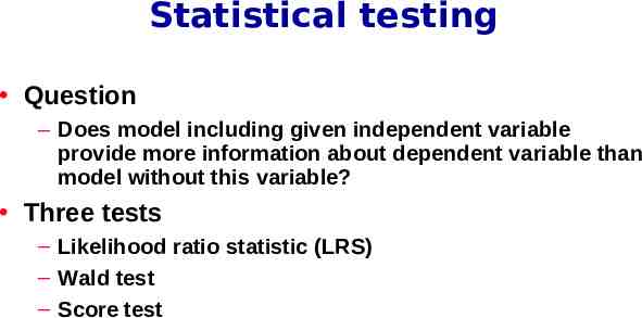
Statistical testing Question – Does model including given independent variable provide more information about dependent variable than model without this variable? Three tests – Likelihood ratio statistic (LRS) – Wald test – Score test
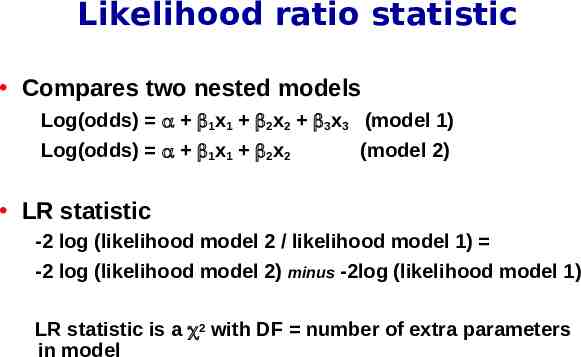
Likelihood ratio statistic Compares two nested models Log(odds) 1x1 2x2 3x3 (model 1) Log(odds) 1x1 2x2 (model 2) LR statistic -2 log (likelihood model 2 / likelihood model 1) -2 log (likelihood model 2) minus -2log (likelihood model 1) LR statistic is a 2 with DF number of extra parameters in model
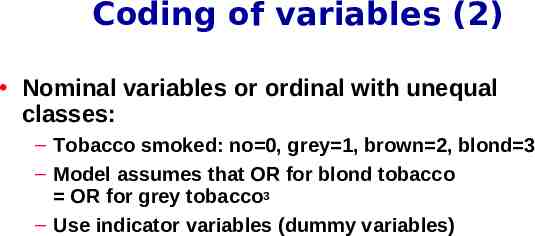
Coding of variables (2) Nominal variables or ordinal with unequal classes: – Tobacco smoked: no 0, grey 1, brown 2, blond 3 – Model assumes that OR for blond tobacco OR for grey tobacco3 – Use indicator variables (dummy variables)
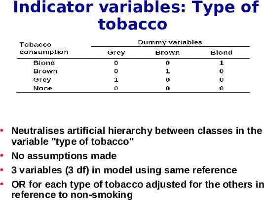
Indicator variables: Type of tobacco Neutralises artificial hierarchy between classes in the variable "type of tobacco" No assumptions made 3 variables (3 df) in model using same reference OR for each type of tobacco adjusted for the others in reference to non-smoking
Reference Hosmer DW, Lemeshow S. Applied logistic regression. Wiley & Sons, New York, 1989
Logistic regression Synthesis
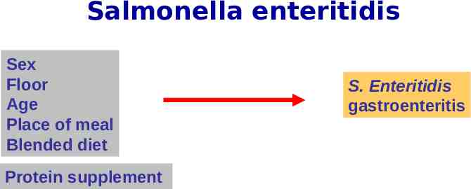
Salmonella enteritidis Sex Floor Age Place of meal Blended diet Protein supplement S. Enteritidis gastroenteritis
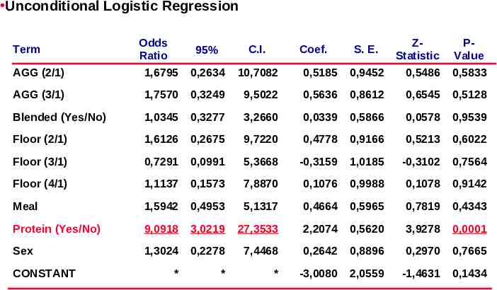
Unconditional Logistic Regression Term Odds Ratio 95% C.I. Coef. S. E. ZStatistic PValue AGG (2/1) 1,6795 0,2634 10,7082 0,5185 0,9452 0,5486 0,5833 AGG (3/1) 1,7570 0,3249 9,5022 0,5636 0,8612 0,6545 0,5128 Blended (Yes/No) 1,0345 0,3277 3,2660 0,0339 0,5866 0,0578 0,9539 Floor (2/1) 1,6126 0,2675 9,7220 0,4778 0,9166 0,5213 0,6022 Floor (3/1) 0,7291 0,0991 5,3668 -0,3159 1,0185 -0,3102 0,7564 Floor (4/1) 1,1137 0,1573 7,8870 0,1076 0,9988 0,1078 0,9142 Meal 1,5942 0,4953 5,1317 0,4664 0,5965 0,7819 0,4343 Protein (Yes/No) 9,0918 3,0219 27,3533 2,2074 0,5620 3,9278 0,0001 Sex 1,3024 0,2278 7,4468 0,2642 0,8896 0,2970 0,7665 * * * -3,0080 2,0559 -1,4631 0,1434 CONSTANT
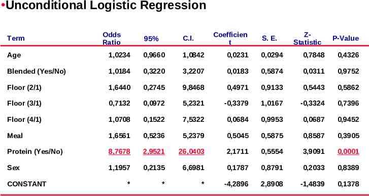
Unconditional Logistic Regression Term Odds Ratio 95% C.I. Coefficien t S. E. ZStatistic P-Value Age 1,0234 0,9660 1,0842 0,0231 0,0294 0,7848 0,4326 Blended (Yes/No) 1,0184 0,3220 3,2207 0,0183 0,5874 0,0311 0,9752 Floor (2/1) 1,6440 0,2745 9,8468 0,4971 0,9133 0,5443 0,5862 Floor (3/1) 0,7132 0,0972 5,2321 -0,3379 1,0167 -0,3324 0,7396 Floor (4/1) 1,0708 0,1522 7,5322 0,0684 0,9953 0,0687 0,9452 Meal 1,6561 0,5236 5,2379 0,5045 0,5875 0,8587 0,3905 Protein (Yes/No) 8,7678 2,9521 26,0403 2,1711 0,5554 3,9091 0,0001 Sex 1,1957 0,2135 6,6981 0,1787 0,8791 0,2033 0,8389 * * * -4,2896 2,8908 -1,4839 0,1378 CONSTANT
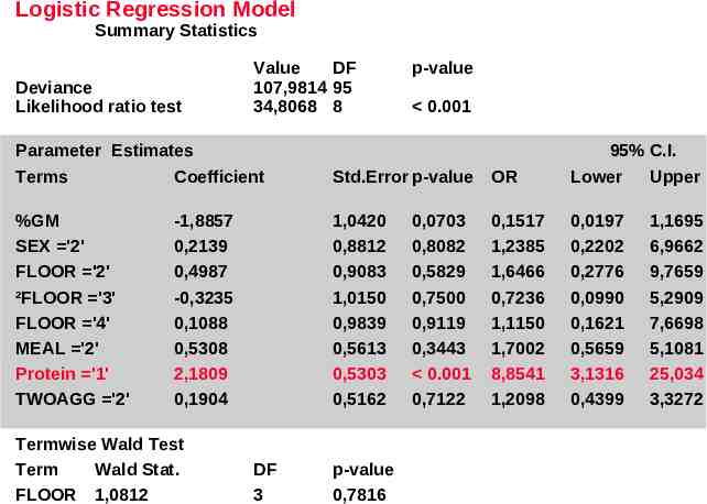
Logistic Regression Model Summary Statistics Deviance Likelihood ratio test Value DF 107,9814 95 34,8068 8 p-value 0.001 Parameter Estimates Terms Coefficient Std.Error p-value OR 95% C.I. Lower Upper %GM SEX '2' FLOOR '2' ²FLOOR '3' FLOOR '4' MEAL '2' Protein '1' TWOAGG '2' 1,0420 0,8812 0,9083 1,0150 0,9839 0,5613 0,5303 0,5162 0,1517 1,2385 1,6466 0,7236 1,1150 1,7002 8,8541 1,2098 0,0197 0,2202 0,2776 0,0990 0,1621 0,5659 3,1316 0,4399 -1,8857 0,2139 0,4987 -0,3235 0,1088 0,5308 2,1809 0,1904 Termwise Wald Test Term Wald Stat. FLOOR 1,0812 DF 3 p-value 0,7816 0,0703 0,8082 0,5829 0,7500 0,9119 0,3443 0.001 0,7122 1,1695 6,9662 9,7659 5,2909 7,6698 5,1081 25,034 3,3272
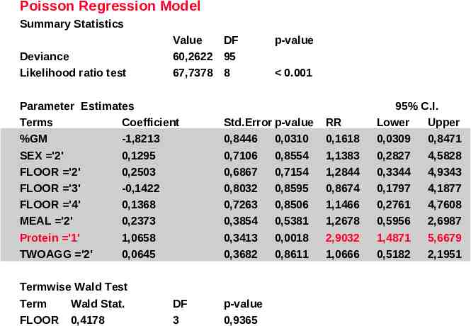
Poisson Regression Model Summary Statistics Deviance Likelihood ratio test Value DF 60,2622 95 67,7378 8 p-value 0.001 Parameter Estimates Terms Coefficient %GM -1,8213 SEX '2' 0,1295 FLOOR '2' 0,2503 FLOOR '3' -0,1422 FLOOR '4' 0,1368 MEAL '2' 0,2373 Protein '1' 1,0658 TWOAGG '2' 0,0645 Std.Error p-value 0,8446 0,0310 0,7106 0,8554 0,6867 0,7154 0,8032 0,8595 0,7263 0,8506 0,3854 0,5381 0,3413 0,0018 0,3682 0,8611 Termwise Wald Test Term Wald Stat. FLOOR 0,4178 p-value 0,9365 DF 3 RR 0,1618 1,1383 1,2844 0,8674 1,1466 1,2678 2,9032 1,0666 95% C.I. Lower Upper 0,0309 0,8471 0,2827 4,5828 0,3344 4,9343 0,1797 4,1877 0,2761 4,7608 0,5956 2,6987 1,4871 5,6679 0,5182 2,1951
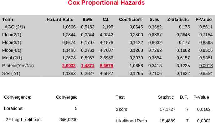
Cox Proportional Hazards Term Hazard Ratio 95% C.I. Coefficient S. E. Z-Statistic P-Value AGG (2/1) 1,0666 0,5183 2,195 0,0645 0,3682 0,175 0,8611 Floor(2/1) 1,2844 0,3344 4,9342 0,2503 0,6867 0,3646 0,7154 Floor(3/1) 0,8674 0,1797 4,1876 -0,1422 0,8032 -0,177 0,8595 Floor(4/1) 1,1466 0,2761 4,7607 0,1368 0,7263 0,1883 0,8506 Meal (2/1) 1,2678 0,5957 2,6986 0,2373 0,3854 0,6157 0,5381 Protein(Yes/No) 2,9032 1,4871 5,6678 1,0658 0,3413 3,1225 0,0018 Sex (2/1) 1,1383 0,2827 4,5827 0,1295 0,7106 0,1822 0,8554 Convergence: Iterations: -2 * Log-Likelihood: Converged 5 346,0200 Test Statistic D.F. P-Value Score 17,1727 7 0,0163 Likelihood Ratio 15,4889 7 0,0302