Quantitative Data Analysis Summarizing Data: variables; simple

Quantitative Data Analysis Summarizing Data: variables; simple statistics; effect statistics and statistical models; complex models. Generalizing from Sample to Population: precision of estimate, confidence limits, statistical significance, p value, errors. Will G Hopkins Auckland University of Technology Auckland NZ Reference: Hopkins WG (2002). Quantitative data analysis (Slideshow). Sportscience 6, sportsci.org/jour/0201/Quantitative analysis.ppt (2046 words)

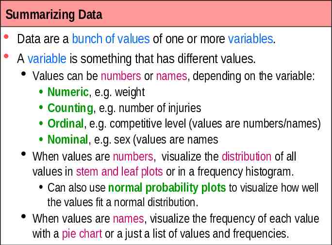
Summarizing Data Data are a bunch of values of one or more variables. A variable is something that has different values. Values can be numbers or names, depending on the variable: Numeric, e.g. weight Counting, e.g. number of injuries Ordinal, e.g. competitive level (values are numbers/names) Nominal, e.g. sex (values are names When values are numbers, visualize the distribution of all values in stem and leaf plots or in a frequency histogram. Can also use normal probability plots to visualize how well the values fit a normal distribution. When values are names, visualize the frequency of each value with a pie chart or a just a list of values and frequencies.

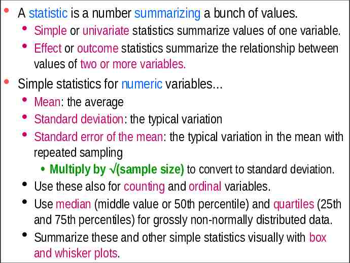
A statistic is a number summarizing a bunch of values. Simple or univariate statistics summarize values of one variable. Effect or outcome statistics summarize the relationship between values of two or more variables. Simple statistics for numeric variables Mean: the average Standard deviation: the typical variation Standard error of the mean: the typical variation in the mean with repeated sampling Multiply by (sample size) to convert to standard deviation. Use these also for counting and ordinal variables. Use median (middle value or 50th percentile) and quartiles (25th and 75th percentiles) for grossly non-normally distributed data. Summarize these and other simple statistics visually with box and whisker plots.

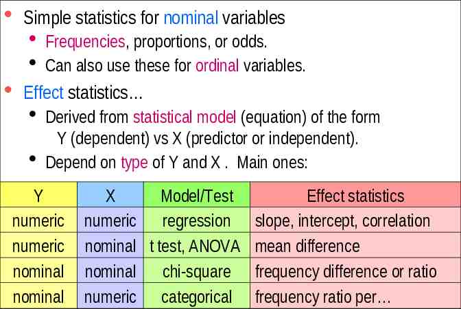
Simple statistics for nominal variables Frequencies, proportions, or odds. Can also use these for ordinal variables. Effect statistics Derived from statistical model (equation) of the form Y (dependent) vs X (predictor or independent). Depend on type of Y and X . Main ones: Y numeric numeric nominal nominal X Model/Test numeric regression nominal t test, ANOVA nominal chi-square numeric categorical Effect statistics slope, intercept, correlation mean difference frequency difference or ratio frequency ratio per

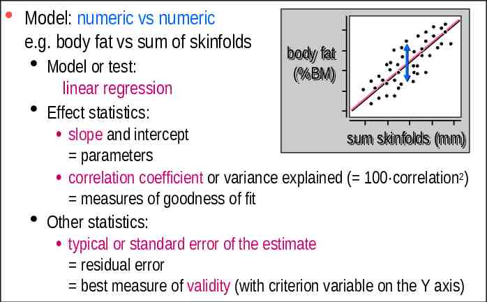
Model: numeric vs numeric e.g. body fat vs sum of skinfolds body fat (%BM) Model or test: linear regression Effect statistics: slope and intercept sum skinfolds (mm) parameters correlation coefficient or variance explained ( 100·correlation2) measures of goodness of fit Other statistics: typical or standard error of the estimate residual error best measure of validity (with criterion variable on the Y axis)

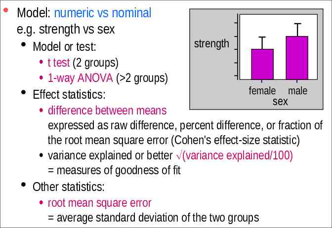
Model: numeric vs nominal e.g. strength vs sex strength Model or test: t test (2 groups) 1-way ANOVA ( 2 groups) female male Effect statistics: sex difference between means expressed as raw difference, percent difference, or fraction of the root mean square error (Cohen's effect-size statistic) variance explained or better (variance explained/100) measures of goodness of fit Other statistics: root mean square error average standard deviation of the two groups

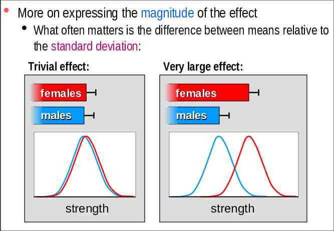
More on expressing the magnitude of the effect What often matters is the difference between means relative to the standard deviation: Trivial effect: Very large effect: females females males males strength strength

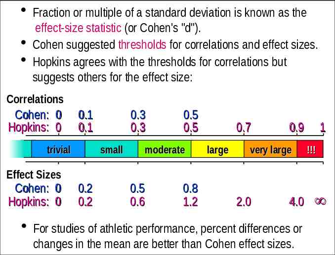
Fraction or multiple of a standard deviation is known as the effect-size statistic (or Cohen's "d"). Cohen suggested thresholds for correlations and effect sizes. Hopkins agrees with the thresholds for correlations but suggests others for the effect size: Correlations Cohen: 0 Hopkins: 0 0.1 0.1 trivial Effect Sizes Cohen: 0 Hopkins: 0 0.3 0.3 small 0.2 0.2 0.5 0.5 moderate 0.5 0.6 0.8 1.2 0.7 large 0.9 very large 2.0 4.0 For studies of athletic performance, percent differences or changes in the mean are better than Cohen effect sizes. 1 !!!

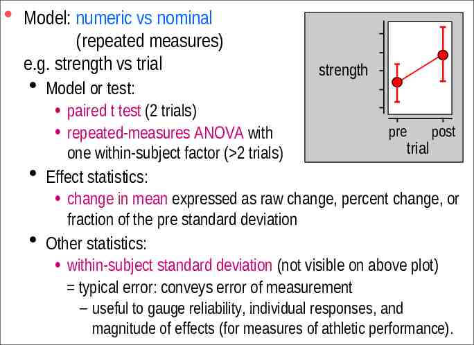
Model: numeric vs nominal (repeated measures) e.g. strength vs trial strength Model or test: paired t test (2 trials) pre post repeated-measures ANOVA with trial one within-subject factor ( 2 trials) Effect statistics: change in mean expressed as raw change, percent change, or fraction of the pre standard deviation Other statistics: within-subject standard deviation (not visible on above plot) typical error: conveys error of measurement – useful to gauge reliability, individual responses, and magnitude of effects (for measures of athletic performance).

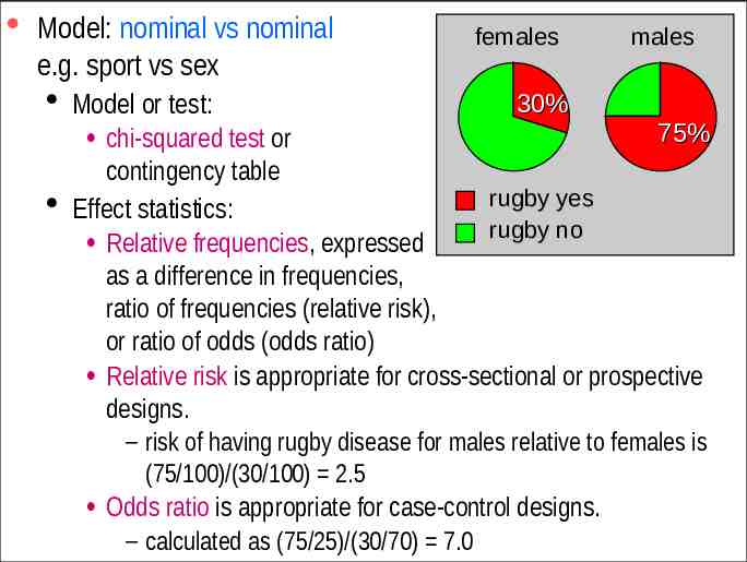
Model: nominal vs nominal e.g. sport vs sex females males Model or test: 30% 75% chi-squared test or contingency table rugby yes Effect statistics: rugby no Relative frequencies, expressed as a difference in frequencies, ratio of frequencies (relative risk), or ratio of odds (odds ratio) Relative risk is appropriate for cross-sectional or prospective designs. – risk of having rugby disease for males relative to females is (75/100)/(30/100) 2.5 Odds ratio is appropriate for case-control designs. – calculated as (75/25)/(30/70) 7.0

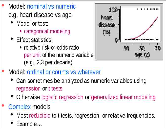
Model: nominal vs numeric e.g. heart disease vs age Model or test: categorical modeling Effect statistics: relative risk or odds ratio per unit of the numeric variable (e.g., 2.3 per decade) 100 heart disease (%) 0 30 50 70 age (y) Model: ordinal or counts vs whatever Can sometimes be analyzed as numeric variables using regression or t tests Otherwise logistic regression or generalized linear modeling Complex models Most reducible to t tests, regression, or relative frequencies. Example

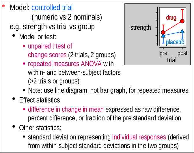
Model: controlled trial (numeric vs 2 nominals) e.g. strength vs trial vs group drug strength Model or test: placebo unpaired t test of pre post change scores (2 trials, 2 groups) trial repeated-measures ANOVA with within- and between-subject factors ( 2 trials or groups) Note: use line diagram, not bar graph, for repeated measures. Effect statistics: difference in change in mean expressed as raw difference, percent difference, or fraction of the pre standard deviation Other statistics: standard deviation representing individual responses (derived from within-subject standard deviations in the two groups)

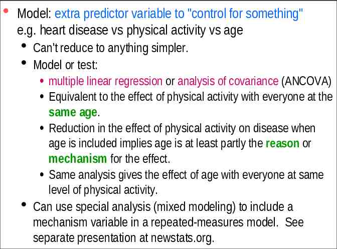
Model: extra predictor variable to "control for something" e.g. heart disease vs physical activity vs age Can't reduce to anything simpler. Model or test: multiple linear regression or analysis of covariance (ANCOVA) Equivalent to the effect of physical activity with everyone at the same age. Reduction in the effect of physical activity on disease when age is included implies age is at least partly the reason or mechanism for the effect. Same analysis gives the effect of age with everyone at same level of physical activity. Can use special analysis (mixed modeling) to include a mechanism variable in a repeated-measures model. See separate presentation at newstats.org.

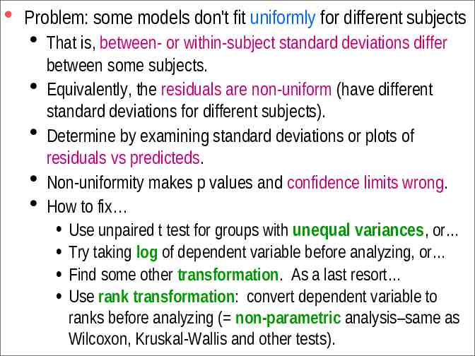
Problem: some models don't fit uniformly for different subjects That is, between- or within-subject standard deviations differ between some subjects. Equivalently, the residuals are non-uniform (have different standard deviations for different subjects). Determine by examining standard deviations or plots of residuals vs predicteds. Non-uniformity makes p values and confidence limits wrong. How to fix Use unpaired t test for groups with unequal variances, or Try taking log of dependent variable before analyzing, or Find some other transformation. As a last resort Use rank transformation: convert dependent variable to ranks before analyzing ( non-parametric analysis–same as Wilcoxon, Kruskal-Wallis and other tests).

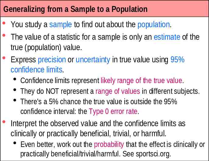
Generalizing from a Sample to a Population You study a sample to find out about the population. The value of a statistic for a sample is only an estimate of the true (population) value. Express precision or uncertainty in true value using 95% confidence limits. Confidence limits represent likely range of the true value. They do NOT represent a range of values in different subjects. There's a 5% chance the true value is outside the 95% confidence interval: the Type 0 error rate. Interpret the observed value and the confidence limits as clinically or practically beneficial, trivial, or harmful. Even better, work out the probability that the effect is clinically or practically beneficial/trivial/harmful. See sportsci.org.

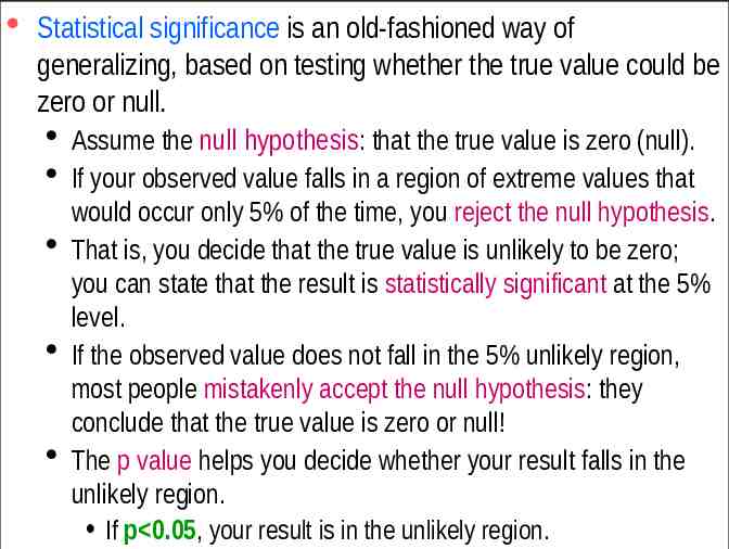
Statistical significance is an old-fashioned way of generalizing, based on testing whether the true value could be zero or null. Assume the null hypothesis: that the true value is zero (null). If your observed value falls in a region of extreme values that would occur only 5% of the time, you reject the null hypothesis. That is, you decide that the true value is unlikely to be zero; you can state that the result is statistically significant at the 5% level. If the observed value does not fall in the 5% unlikely region, most people mistakenly accept the null hypothesis: they conclude that the true value is zero or null! The p value helps you decide whether your result falls in the unlikely region. If p 0.05, your result is in the unlikely region.

One meaning of the p value: the probability of a more extreme observed value (positive or negative) when true value is zero. Better meaning of the p value: if you observe a positive effect, 1 - p/2 is the chance the true value is positive, and p/2 is the chance the true value is negative. Ditto for a negative effect. Example: you observe a 1.5% enhancement of performance (p 0.08). Therefore there is a 96% chance that the true effect is any "enhancement" and a 4% chance that the true effect is any "impairment". This interpretation does not take into account trivial enhancements and impairments. Therefore, if you must use p values, show exact values, not p 0.05 or p 0.05. Meta-analysts also need the exact p value (or confidence limits).

If the true value is zero, there's a 5% chance of getting statistical significance: the Type I error rate, or rate of false positives or false alarms. There's also a chance that the smallest worthwhile true value will produce an observed value that is not statistically significant: the Type II error rate, or rate of false negatives or failed alarms. In the old-fashioned approach to research design, you are supposed to have enough subjects to make a Type II error rate of 20%: that is, your study is supposed to have a power of 80% to detect the smallest worthwhile effect. If you look at lots of effects in a study, there's an increased chance being wrong about at least one of them. Old-fashioned statisticians like to control this inflation of the Type I error rate within an ANOVA to make sure the increased chance is kept to 5%. This approach is misguided.

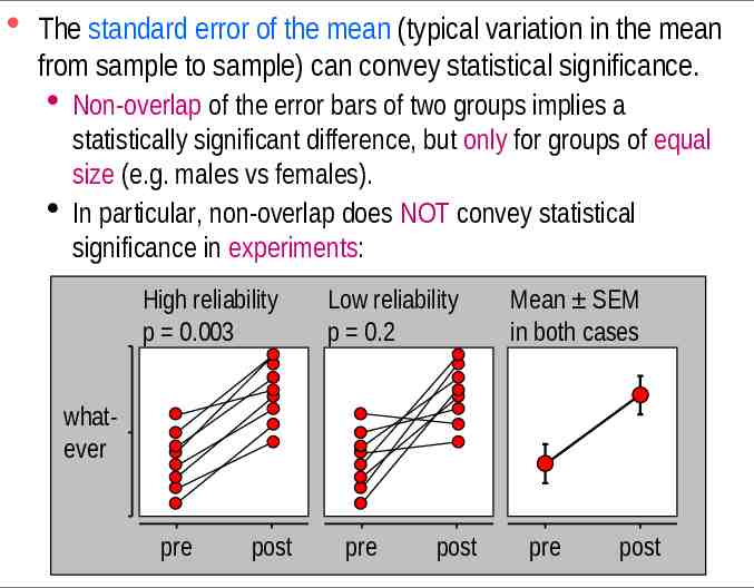
The standard error of the mean (typical variation in the mean from sample to sample) can convey statistical significance. Non-overlap of the error bars of two groups implies a statistically significant difference, but only for groups of equal size (e.g. males vs females). In particular, non-overlap does NOT convey statistical significance in experiments: High reliability p 0.003 Low reliability p 0.2 Mean SEM in both cases whatever pre post pre post pre post

In summary If you must use statistical significance, show exact p values. Better still, show confidence limits instead. NEVER show the standard error of the mean! Show the usual between-subject standard deviation to convey the spread between subjects. In population studies, this standard deviation helps convey magnitude of differences or changes in the mean. In interventions, show also the within-subject standard deviation (the typical error) to convey precision of measurement. In athlete studies, this standard deviation helps convey magnitude of differences or changes in mean performance.