Probability and Statistics in Engineering Philip Bedient, Ph.D.

Probability and Statistics in Engineering Philip Bedient, Ph.D.

Probability: Basic Ideas Terminology: Trial: each time you repeat an experiment Outcome: result of an experiment Random experiment: one with random outcomes (cannot be predicted exactly) Relative frequency: how many times a specific outcome occurs within the entire experiment.

Statistics: Basic Ideas Statistics is the area of science that deals with collection, organization, analysis, and interpretation of data. It also deals with methods and techniques that can be used to draw conclusions about the characteristics of a large number of data points-commonly called a population-By using a smaller subset of the entire data.

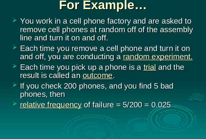
For Example You work in a cell phone factory and are asked to remove cell phones at random off of the assembly line and turn it on and off. Each time you remove a cell phone and turn it on and off, you are conducting a random experiment. Each time you pick up a phone is a trial and the result is called an outcome. If you check 200 phones, and you find 5 bad phones, then relative frequency of failure 5/200 0.025

Statistics in Engineering Engineers apply physical and chemical laws and mathematics to design, develop, test, and supervise various products and services. Engineers perform tests to learn how things behave under stress, and at what point they might fail.

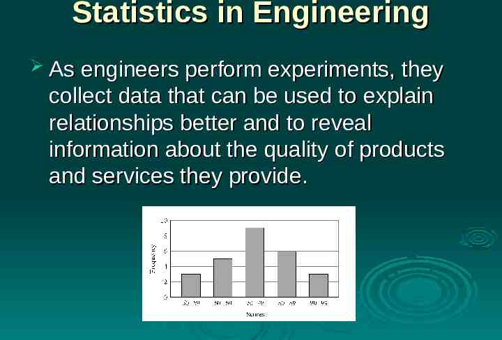
Statistics in Engineering As engineers perform experiments, they collect data that can be used to explain relationships better and to reveal information about the quality of products and services they provide.

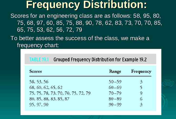
Frequency Distribution: Scores for an engineering class are as follows: 58, 95, 80, 75, 68, 97, 60, 85, 75, 88, 90, 78, 62, 83, 73, 70, 70, 85, 65, 75, 53, 62, 56, 72, 79 To better assess the success of the class, we make a frequency chart:

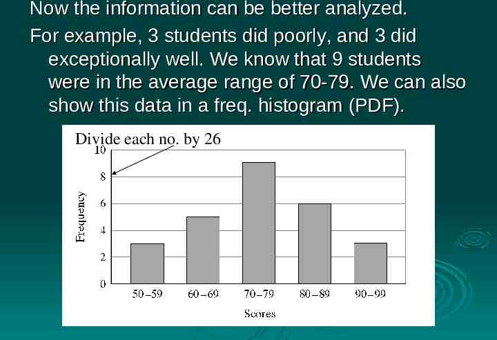
Now the information can be better analyzed. For example, 3 students did poorly, and 3 did exceptionally well. We know that 9 students were in the average range of 70-79. We can also show this data in a freq. histogram (PDF). Divide each no. by 26

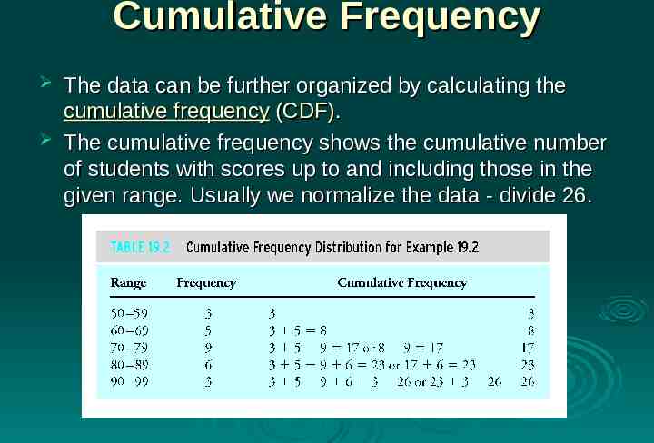
Cumulative Frequency The data can be further organized by calculating the cumulative frequency (CDF). The cumulative frequency shows the cumulative number of students with scores up to and including those in the given range. Usually we normalize the data - divide 26.

Measures of Central Tendency & Variation Systematic errors, also called fixed errors, are errors associated with using an inaccurate instrument. These errors can be detected and avoided by properly calibrating instruments Random errors are generated by a number of unpredictable variations in a given measurement situation. Mechanical vibrations of instruments or variations in line voltage friction or humidity could lead to random fluctuations in observations.

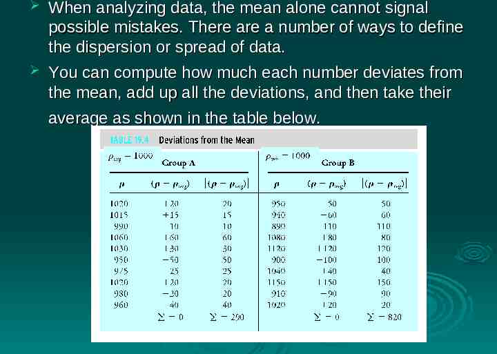
When analyzing data, the mean alone cannot signal possible mistakes. There are a number of ways to define the dispersion or spread of data. You can compute how much each number deviates from the mean, add up all the deviations, and then take their average as shown in the table below.

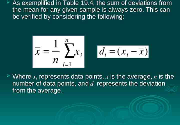
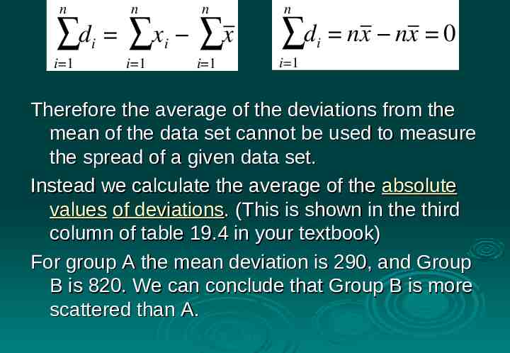
As exemplified in Table 19.4, the sum of deviations from the mean for any given sample is always zero. This can be verified by considering the following: n 1 x x i n i 1 di (x i x ) Where xi represents data points, x is the average, n is the number of data points, and d, represents the deviation from the average.

n n n n d x x d i 1 i 1 i i i 1 i 1 i nx nx 0 Therefore the average of the deviations from the mean of the data set cannot be used to measure the spread of a given data set. Instead we calculate the average of the absolute values of deviations. (This is shown in the third column of table 19.4 in your textbook) For group A the mean deviation is 290, and Group B is 820. We can conclude that Group B is more scattered than A.

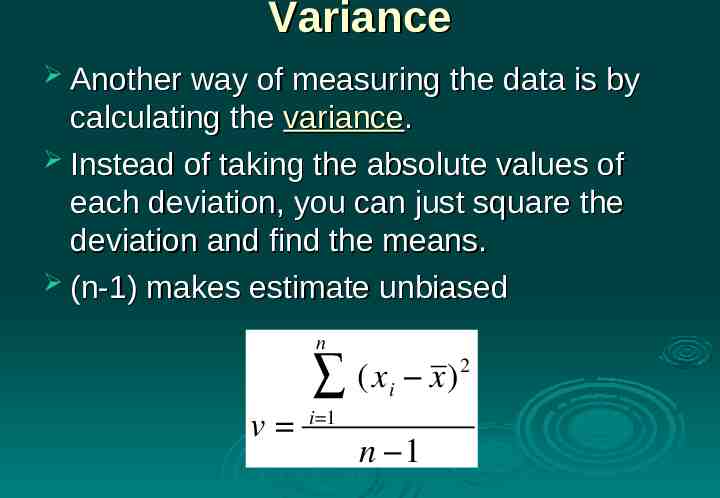
Variance Another way of measuring the data is by calculating the variance. Instead of taking the absolute values of each deviation, you can just square the deviation and find the means. (n-1) makes estimate unbiased n (x v i x) i 1 n 1 2

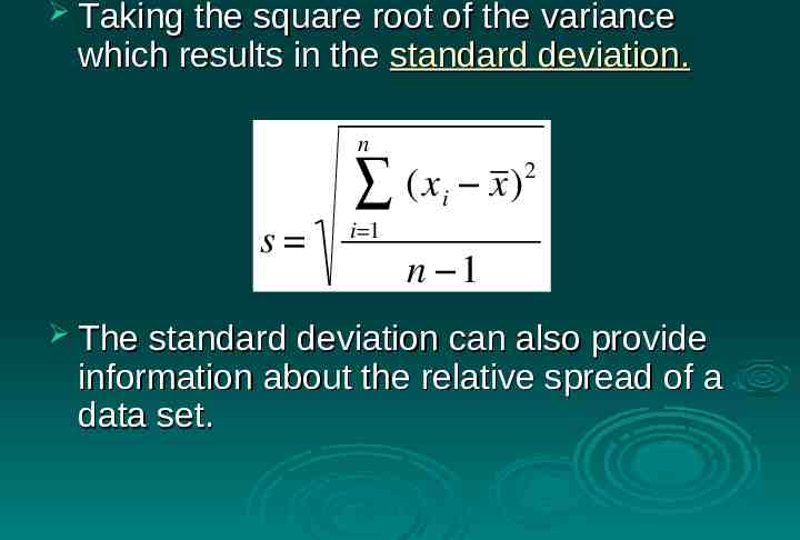
Taking the square root of the variance which results in the standard deviation. n (x s i x) 2 i 1 n 1 The standard deviation can also provide information about the relative spread of a data set.

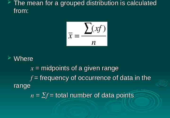
The mean for a grouped distribution is calculated from: (xf ) x n Where x midpoints of a given range f frequency of occurrence of data in the range n f total number of data points

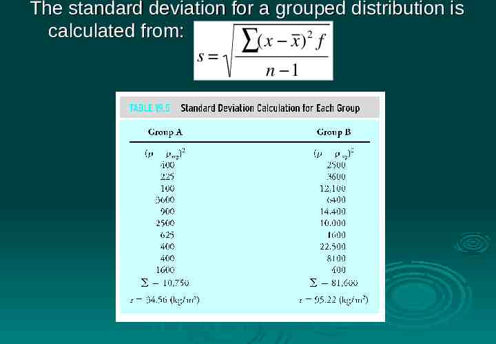
The standard deviation for a grouped distribution is calculated from: 2 (x x ) f s n 1

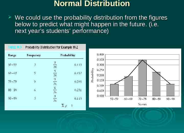
Normal Distribution We could use the probability distribution from the figures below to predict what might happen in the future. (i.e. next year’s students’ performance)

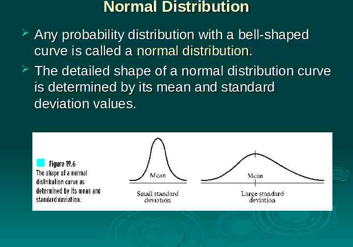
Normal Distribution Any probability distribution with a bell-shaped curve is called a normal distribution. The detailed shape of a normal distribution curve is determined by its mean and standard deviation values.

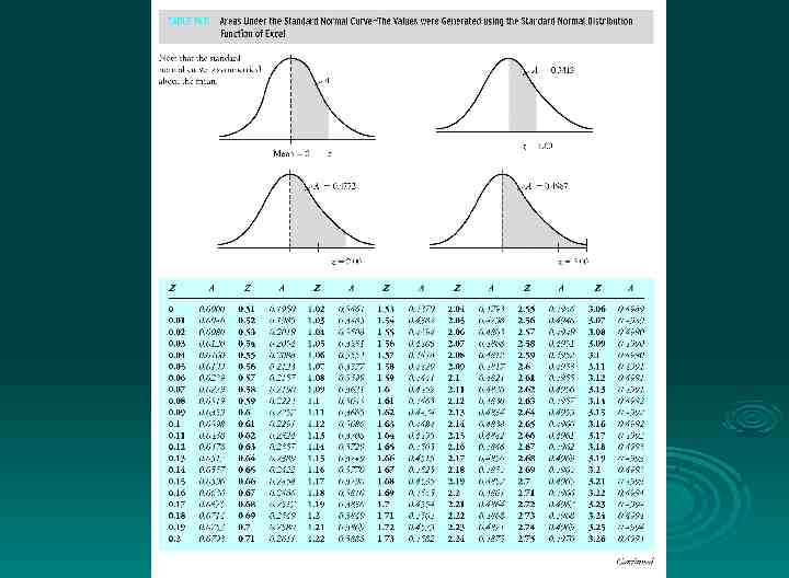
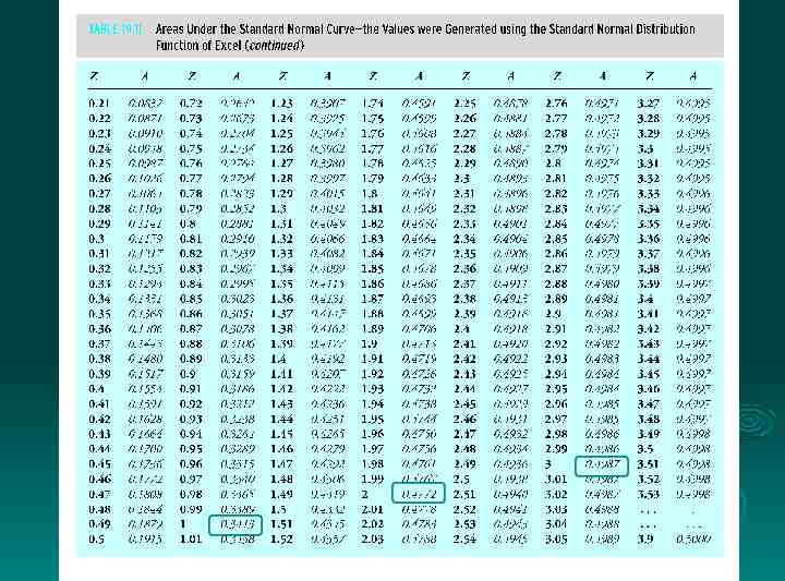
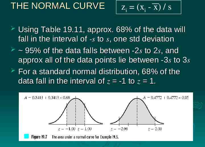
THE NORMAL CURVE zi (xi - x) / s Using Table 19.11, approx. 68% of the data will fall in the interval of -s to s, one std deviation 95% of the data falls between -2s to 2s, and approx all of the data points lie between -3 s to 3s For a standard normal distribution, 68% of the data fall in the interval of z -1 to z 1.

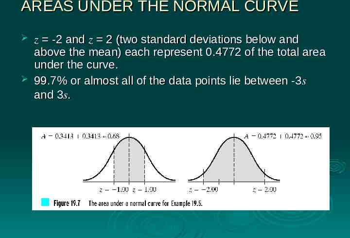
AREAS UNDER THE NORMAL CURVE z -2 and z 2 (two standard deviations below and above the mean) each represent 0.4772 of the total area under the curve. 99.7% or almost all of the data points lie between -3s and 3s.

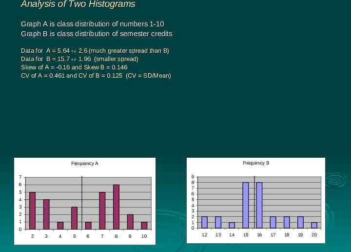
Analysis of Two Histograms Graph A is class distribution of numbers 1-10 Graph B is class distribution of semester credits Data for A 5.64 /- 2.6 (much greater spread than B) Data for B 15.7 /- 1.96 (smaller spread) Skew of A -0.16 and Skew B 0.146 CV of A 0.461 and CV of B 0.125 (CV SD/Mean) Frequency B Frequency A 9 8 7 6 5 4 3 2 1 0 7 6 5 4 3 2 1 0 2 3 4 5 6 7 8 9 10 12 13 14 15 16 17 18 19 20